R Basics

Review of basic syntax in R

Figure 1: Figure from https://www.phdcomics.com/comics/archive/phd031714s.gif

Load Packages

library(tidyverse)
theme_set(theme_classic() +
    theme(panel.grid.major.y = element_line(color = "grey92")))

Create an Object and Get Object Information

# Create an object named `x`, using the assignment operator `<-`
x <- c(1, 2)
# Generally, nothing returns after an assignment. Type `x` to print the object
x

#> [1] 1 2

# Check the type
typeof(x)

#> [1] "double"

# Check the length
length(x)

#> [1] 2

# A quick look of the structure of an object
str(x)

#>  num [1:2] 1 2

Another example

y <- as.character(c(seq(1, to = 10, by = 0.5), 99, 99))
typeof(y)

#> [1] "character"

str(y)

#>  chr [1:21] "1" "1.5" "2" "2.5" "3" "3.5" "4" "4.5" "5" "5.5" "6" ...

To find out what the seq() function does, use

?seq

Piping

A pipe operator is an alternative way to do multiple operations on an object. For example, the following code (a) transforms y to numbers, (b) recodes the value 99 to missing, and (c) obtains the mean. The traditional way to do it in R is through nested parentheses:

# 3. Get the mean
mean(
    # 2. Recode 99 to missing
    na_if(
        # 1. transform to numbers
        as.numeric(y), 99
    ),
    na.rm = TRUE
)

#> [1] 5.5

What’s inconvenient is that the last operation needs to be put first. Also, it’s hard to keep track of the parentheses. Some users, including myself, prefer the alternative way of doing the same as the above code:

y %>%
    # 1. transform to numbers
    as.numeric() %>%
    # 2. Recode 99 to missing
    na_if(99) %>%
    # 3. Get the mean
    mean(na.rm = TRUE)

#> [1] 5.5

The pipe operator works by taking the object before %>% as the first argument for the function after %>%. So y %>% as.numeric() is the same as as.numeric(y), and y2 %>% na_if(99) is the same as na_if(y2, 99).

The %>% operator requires loading the tidyverse package (specifically magrittr package). Since R 4.1.0, one can use |> for piping without loading any packages. While in the future, |> may be the preferred way, for now, we’ll stick to %>% to make things compatible for older versions of R.

Vector, Matrix, Array, List, and Data Frames

# Vector
(vector_a <- 1:10)

#>  [1]  1  2  3  4  5  6  7  8  9 10

typeof(vector_a)

#> [1] "integer"

is.vector(vector_a)  # check whether it is a vector

#> [1] TRUE

vector_a[2:3]  # select the second and the third elements

#> [1] 2 3

(vector_b <- c("classical", "frequentisti", "Bayesian"))

#> [1] "classical"    "frequentisti" "Bayesian"

typeof(vector_b)  # character vector

#> [1] "character"

logical_b <- vector_b == "Bayesian"
typeof(logical_b)  # logical vector

#> [1] "logical"

# Matrix
matrix_c <- matrix(1:10, nrow = 5, ncol = 2)
rownames(matrix_c) <- paste0("row", 1:5)
colnames(matrix_c) <- c("var1", "var2")
matrix_c

#>      var1 var2
#> row1    1    6
#> row2    2    7
#> row3    3    8
#> row4    4    9
#> row5    5   10

typeof(matrix_c)

#> [1] "integer"

class(matrix_c)

#> [1] "matrix" "array"

str(matrix_c)

#>  int [1:5, 1:2] 1 2 3 4 5 6 7 8 9 10
#>  - attr(*, "dimnames")=List of 2
#>   ..$ : chr [1:5] "row1" "row2" "row3" "row4" ...
#>   ..$ : chr [1:2] "var1" "var2"

is.vector(matrix_c)  # check whether it is a vector

#> [1] FALSE

is.matrix(matrix_c)  # check whether it is a matrix

#> [1] TRUE

matrix_c[c("row1", "row5"), ]  # select rows 1 and 5

#>      var1 var2
#> row1    1    6
#> row5    5   10

matrix_c[, 1]  # select first column (converted to a vector)

#> row1 row2 row3 row4 row5 
#>    1    2    3    4    5

set.seed(123)  # for reproducibility
# Array: An array can have one, two, or more dimensions. 
# A matrix is also an array.
array_d <- array(rnorm(8), dim = c(2, 2, 2))
array_d

#> , , 1
#> 
#>            [,1]       [,2]
#> [1,] -0.5604756 1.55870831
#> [2,] -0.2301775 0.07050839
#> 
#> , , 2
#> 
#>           [,1]       [,2]
#> [1,] 0.1292877  0.4609162
#> [2,] 1.7150650 -1.2650612

str(array_d)

#>  num [1:2, 1:2, 1:2] -0.5605 -0.2302 1.5587 0.0705 0.1293 ...

typeof(array_d)  # numeric type

#> [1] "double"

class(array_d)

#> [1] "array"

is.matrix(array_d)

#> [1] FALSE

is.array(array_d)

#> [1] TRUE

array_d[1, 1,]  # use 3 indices for a 3-D array

#> [1] -0.5604756  0.1292877

# List
# An array is a vector where each component can have a different type
list_e <- list("abc", 5, 2.57, TRUE)
typeof(list_e)

#> [1] "list"

class(list_e)  # `list` for both type of class

#> [1] "list"

str(list_e)

#> List of 4
#>  $ : chr "abc"
#>  $ : num 5
#>  $ : num 2.57
#>  $ : logi TRUE

list_e[1]  # extract first element, and put it in a list

#> [[1]]
#> [1] "abc"

list_e[[1]]  # extract first element

#> [1] "abc"

list_f <- list(name = "abc", age = 5)  # named list
# Can also extract element by name (as opposed to by position)
list_f$name

#> [1] "abc"

is.vector(list_f)  # a one-dimension list is a special type of vector

#> [1] TRUE

# Data Frame
# A data frame is a special type of list with two dimensions.
# It is a list of multiple column vectors
(dataframe_c <- as.data.frame(matrix_c))

#>      var1 var2
#> row1    1    6
#> row2    2    7
#> row3    3    8
#> row4    4    9
#> row5    5   10

typeof(dataframe_c)  # type is list

#> [1] "list"

class(dataframe_c)  # data.frame

#> [1] "data.frame"

dataframe_c[c(1, 2),]  # subset using matrix method

#>      var1 var2
#> row1    1    6
#> row2    2    7

dataframe_c$var1  # extract columns using list method

#> [1] 1 2 3 4 5

dataframe_c[[1]]  # same as above

#> [1] 1 2 3 4 5

# select first column, and put it as a data.frame(list)
dataframe_c[1]

#>      var1
#> row1    1
#> row2    2
#> row3    3
#> row4    4
#> row5    5

Plotting

The popular ggplot2 package uses the “grammar of graphics” approach to plotting. It is an elegant and comprehensive system for graphics but requires mastering some vocabulary. As a quick start, each plot requires specifying

• Some layer(s) of geometric elements (e.g., points, lines, boxplots, etc)
• Mapping of some data/variables to some aesthetic attributes (e.g., axis, color, point shape)

To learn more, please take a look at the cheatsheet: https://www.rstudio.com/resources/cheatsheets/

For example, consider the airquality data set:

head(airquality)

#>   Ozone Solar.R Wind Temp Month Day
#> 1    41     190  7.4   67     5   1
#> 2    36     118  8.0   72     5   2
#> 3    12     149 12.6   74     5   3
#> 4    18     313 11.5   62     5   4
#> 5    NA      NA 14.3   56     5   5
#> 6    28      NA 14.9   66     5   6

One can show the distribution of Ozone. On a 2-D Cartesian coordinate system, if we want to show the data in points, each point needs the x- and the y-coordinates. Therefore, the following gives an error as it only maps Ozone to the x-axis:

ggplot(data = airquality) +
    # Add a layer of points
    geom_point(aes(x = Ozone))

#> Error in `check_required_aesthetics()`:
#> ! geom_point requires the following missing aesthetics: y

While not very interesting, we can instead specify every point to have a y-coordinate of 0:

ggplot(data = airquality) +
    # Add a layer of points
    geom_point(aes(x = Ozone, y = 0))

Some geometric objects (geom) assign the y-coordinate automatically. For example, geom_histogram uses bars, with the x-coordinate based on the variable and the y-coordinate based on the counts of each bin.

ggplot(data = airquality) +
    # Add a layer of a histogram (a set of bars)
    geom_histogram(aes(x = Ozone))

Scatter plot

A scatter plot maps the x- and the y-axes to two variables

ggplot(data = airquality) +
    # Add a layer of a points
    geom_point(aes(x = Wind, y = Ozone),
               # alpha = 0.3 makes points transparent
               alpha = 0.5)

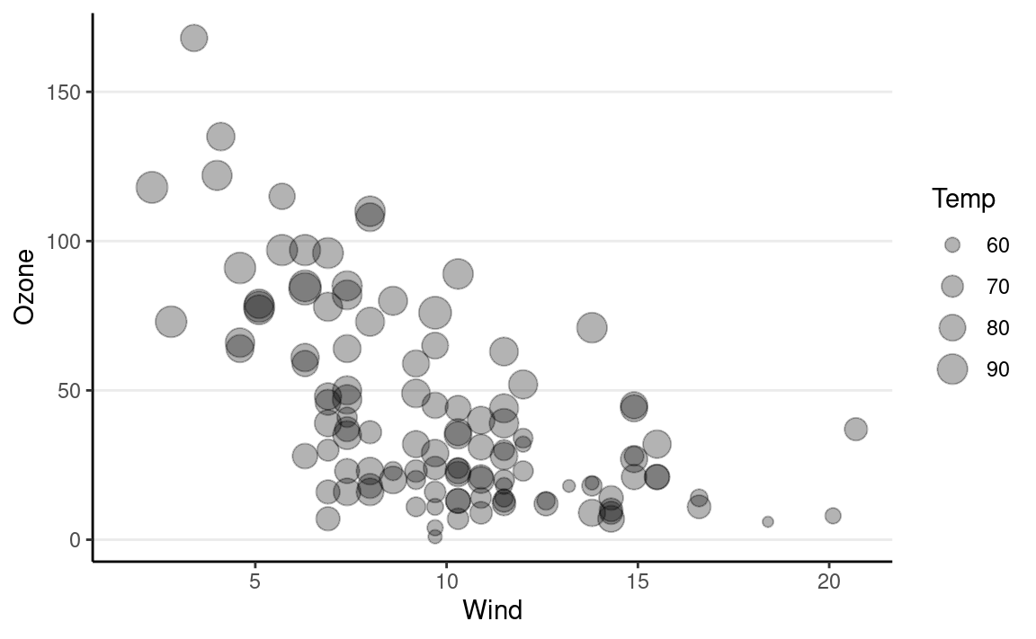
The x- and y-coordinates are not the only attributes for the points geometric object. For example, we can map the sizes of the points to another variable:

ggplot(data = airquality) +
    # Add a layer of a points
    geom_point(aes(x = Wind, y = Ozone, size = Temp),
               alpha = 0.3)

Changing labels

To change the labels of axis and legend, use labs:

ggplot(data = airquality) +
    # Add a layer of a points
    geom_point(aes(x = Wind, y = Ozone, size = Temp),
               alpha = 0.3) +
    labs(x = "Wind (mph)", y = "Ozone (ppb)", size = "Temperature (degree F)")

Different geom

We can use other geometric objects. For example, geom_smooth adds a smoothing trend

# By putting `aes()` in the first line, all subsequent layers use the same
# mapping
ggplot(aes(x = Wind, y = Ozone), data = airquality) +
    # Add a layer of points
    geom_point() +
    # Add a layer of lines
    geom_smooth()

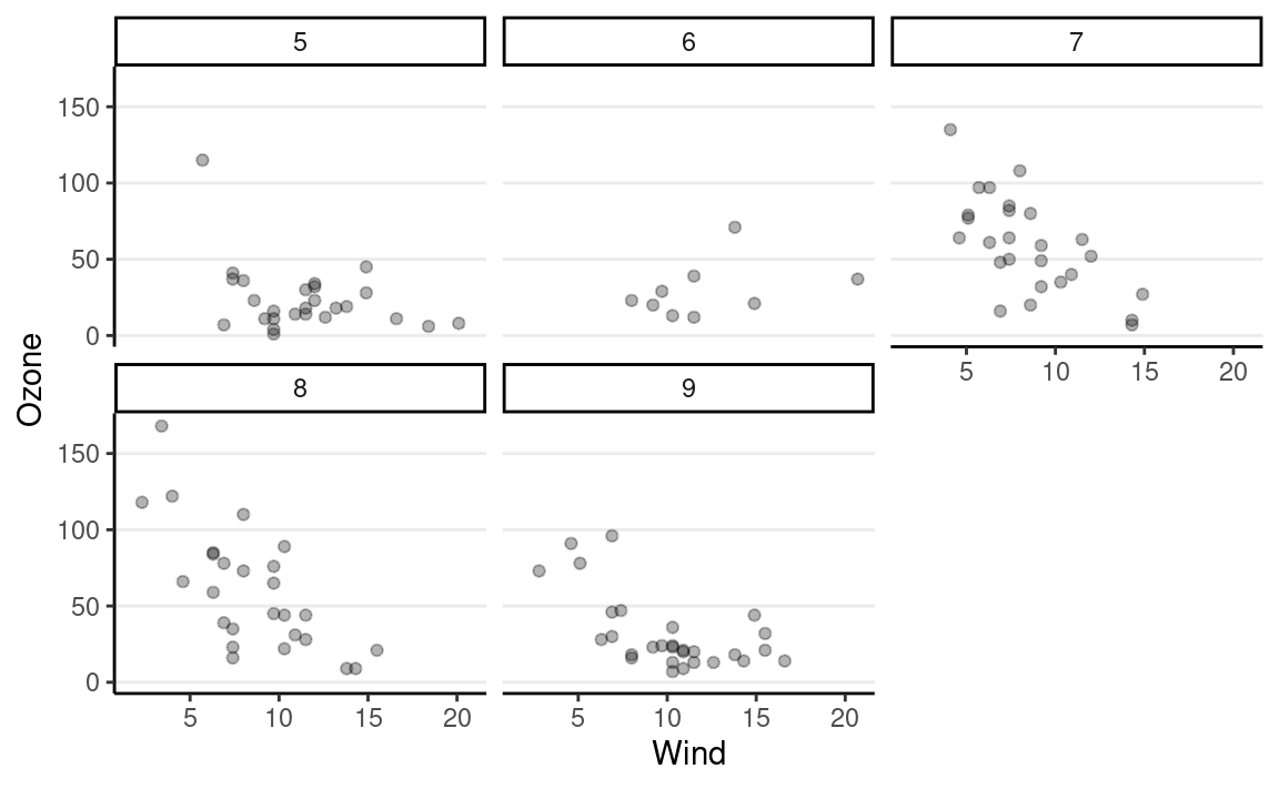
Facet

In many situations, we want to split the data into multiple plots through facet.

ggplot(aes(x = Wind, y = Ozone), data = airquality) +
    # Add a layer of a points
    geom_point(alpha = 0.3) +
    # Split by `Month`
    facet_wrap(~ Month)

for Loop

Using a loop allows one to perform some actions multiple times. See https://r4ds.had.co.nz/iteration.html#introduction-14

The following example shows an example of drawing a random variable from a normal distribution with SD = 1, mean = the previously generated number.

set.seed(2208)  # for reproducibility
# Simulate data
random_numbers <- rep(NA, 100)  # initialize an empty vector
random_numbers[1] <- 10  # set the first value to 10
# i = 2 in the first iteration, then 3, then 4, until i = 100
for (i in 2:100) {
    # `rnorm(1)` simulate one value from a normal distribution;
    # `mean = random_numbers[i - 1]` says the mean of the distribution is
    # from the previously simulated value.
    random_numbers[i] <- rnorm(1, mean = random_numbers[i - 1])
}
# Show the simulated values using ggplot
ggplot(
    tibble(iter = 1:100, random_numbers),
    aes(x = iter, y = random_numbers)
) +
    geom_line() +
    geom_point()

Custom Function

A function in R is a named object that takes in some inputs, performs some operations, and gives some outputs.

Example 1: \(a^2 + b\)

Here is an example of how you can define your own function, from p. 64 of the text

asqplusb <- function(a, b = 1) {
    c <- a ^ 2 + b  # c = a^2 + b
    c  # the last line is usually the output
}

The above function asqplusb() takes two inputs: a and b. The names of these two are called arguments. So we say a and b are the arguments of asqplusb(). We can invoke the function like

asqplusb(2, 3)  # a = 2, b = 3, 2^2 + 3 = 7

#> [1] 7

# This is equivalent to
asqplusb(a = 2, b = 3)

#> [1] 7

# But not the same as
asqplusb(b = 2, a = 3)

#> [1] 11

In the function call, 2 and 3 are the values of the arguments, not the arguments themselves.

Also, when we define the function, we define the first argument as a, and the second argument as b = 1. The latter means the default value of b is 1. So when one calls the function without specifying b, like

asqplusb(4)  # a = 4, b = 1, 4^2 + 1 = 17

#> [1] 17

It is equivalent to

asqplusb(4, b = 1)  # a = 4, b = 1, 4^2 + 1 = 17

#> [1] 17

When to use a function?

Writing one’s own function is very common in R programming, especially with Bayesian analysis, because often one needs to perform some procedures more than once, and it is tedious to write similar code every time. A rule of thumb is that if you have a few lines of code that you find yourself typing more than two times, you should write a function for it. As an example, we can wrap the simulation code above into a function that you can try out with different numbers of iterations:

my_simulate <- function(nsim = 100) {
    # Simulate data
    random_numbers <- rep(NA, nsim) # initialize an empty vector
    random_numbers[1] <- 10 # set the first value to 10
    # i = 2 in the first iteration, then 3, then 4, until i = 100
    for (i in 2:nsim) {
        # `rnorm(1)` simulate one value from a normal distribution;
        # `mean = random_numbers[i - 1]` says the mean of the distribution is
        # from the previously simulated value.
        random_numbers[i] <- rnorm(1, mean = random_numbers[i - 1])
    }
    # Show the simulated values using ggplot
    ggplot(
        tibble(iter = 1:nsim, random_numbers),
        aes(x = iter, y = random_numbers)
    ) +
        geom_line() +
        geom_point()
}

Try to call the above function.

Last updated

#> [1] "January 13, 2022"