library(tidyverse)
library(here)
library(brms)  # simplify fitting Stan GLM models
library(posterior)  # for summarizing draws
library(modelsummary)  # table for brms
theme_set(theme_classic() +
    theme(panel.grid.major.y = element_line(color = "grey92")))
waffle_divorce <- read_delim(  # read delimited files
    "https://raw.githubusercontent.com/rmcelreath/rethinking/master/data/WaffleDivorce.csv",
    delim = ";"
)
# Rescale Marriage and Divorce by dividing by 10
waffle_divorce$Marriage <- waffle_divorce$Marriage / 10
waffle_divorce$Divorce <- waffle_divorce$Divorce / 10
waffle_divorce$MedianAgeMarriage <- waffle_divorce$MedianAgeMarriage / 10
# Recode `South` to a factor variable
waffle_divorce$South <- factor(waffle_divorce$South,
    levels = c(0, 1),
    labels = c("non-south", "south")
)
# See data description at https://rdrr.io/github/rmcelreath/rethinking/man/WaffleDivorce.html
Different Slopes Across Two Groups
Stratified Analysis
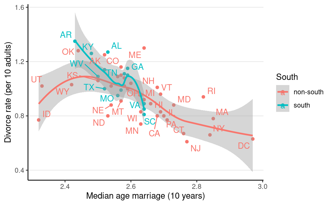
Let’s consider whether the association between
MedianAgeMarriage and Divorce differs between
Southern and non-Southern states. Because (and only
because) the groups are independent, we can
fit a linear regression for each subset of states.
ggplot(waffle_divorce,
       aes(x = MedianAgeMarriage, y = Divorce, col = South)) +
    geom_point() +
    geom_smooth() +
    labs(x = "Median age marriage (10 years)",
         y = "Divorce rate (per 10 adults)") +
    ggrepel::geom_text_repel(aes(label = Loc))
m_nonsouth <-
    brm(Divorce ~ MedianAgeMarriage,
        data = filter(waffle_divorce, South == "non-south"),
        prior = prior(normal(0, 2), class = "b") +
            prior(normal(0, 10), class = "Intercept") +
            prior(student_t(4, 0, 3), class = "sigma"),
        seed = 941,
        iter = 4000
    )
m_south <-
    brm(Divorce ~ MedianAgeMarriage,
        data = filter(waffle_divorce, South == "south"),
        prior = prior(normal(0, 2), class = "b") +
            prior(normal(0, 10), class = "Intercept") +
            prior(student_t(4, 0, 3), class = "sigma"),
        seed = 2157,  # use a different seed
        iter = 4000
    )
msummary(list(South = m_south, `Non-South` = m_nonsouth),
         estimate = "{estimate} [{conf.low}, {conf.high}]",
         statistic = NULL, fmt = 2,
         gof_omit = "^(?!Num)"  # only include number of observations
)
| South | Non-South | |
|---|---|---|
| b_Intercept | 6.09 [3.79, 8.58] | 2.74 [1.77, 3.77] |
| b_MedianAgeMarriage | −1.96 [−2.95, −1.07] | −0.69 [−1.08, −0.32] |
| sigma | 0.11 [0.07, 0.16] | 0.15 [0.12, 0.20] |
| Num.Obs. | 14 | 36 |
We can now ask two questions:
- Is the intercept different across southern and non-southern states?
- Is the slope different across southern and non-southern states?
The correct way to answer the above questions is to obtain the posterior distribution of the difference in the coefficients. Repeat: obtain the posterior distribution of the difference. The incorrect way is to compare whether the CIs overlap.
Here are the posteriors of the differences:
# Extract draws
draws_south <- as_draws_matrix(m_south,
    variable = c("b_Intercept", "b_MedianAgeMarriage")
)
draws_nonsouth <- as_draws_matrix(m_nonsouth,
    variable = c("b_Intercept", "b_MedianAgeMarriage")
)
# Difference in coefficients
draws_diff <- draws_south - draws_nonsouth
# Rename the columns
colnames(draws_diff) <- paste0("d", colnames(draws_diff))
# Summarize
summarize_draws(draws_diff)
#> # A tibble: 2 × 10
#>   variable         mean median    sd   mad    q5    q95  rhat ess_bulk
#>   <chr>           <dbl>  <dbl> <dbl> <dbl> <dbl>  <dbl> <dbl>    <dbl>
#> 1 db_Intercept     3.33   3.34 1.33  1.28   1.16  5.49   1.00    6412.
#> 2 db_MedianAgeMa… -1.27  -1.27 0.519 0.499 -2.11 -0.424  1.00    6411.
#> # … with 1 more variable: ess_tail <dbl>
As you can see, the southern states have a larger intercept and a lower slope.
p1 <- plot(
    conditional_effects(m_nonsouth),
    points = TRUE, plot = FALSE
)[[1]] + ggtitle("Non-South") + lims(x = c(2.3, 3), y = c(0.6, 1.4))
p2 <- plot(
    conditional_effects(m_south),
    points = TRUE, plot = FALSE
)[[1]] + ggtitle("South") + lims(x = c(2.3, 3), y = c(0.6, 1.4))
gridExtra::grid.arrange(p1, p2, ncol = 2)

Interaction Model
An alternative is to include an interaction term
\[ \begin{aligned} D_i & \sim N(\mu_i, \sigma) \\ \mu_i & = \beta_0 + \beta_1 S_i + \beta_2 A_i + \beta_3 S_i \times A_i \\ \beta_0 & \sim N(0, 10) \\ \beta_1 & \sim N(0, 10) \\ \beta_2 & \sim N(0, 1) \\ \beta_3 & \sim N(0, 2) \\ \sigma & \sim t^+_4(0, 3) \end{aligned} \]
- \(\beta_1\): Difference in intercept between southern and non-southern states.
- \(\beta_3\): Difference in the coefficient for A → D between southern and non-southern states
In the model, the variable S, southern state, is a dummy variable with 0 = non-southern and 1 = southern. Therefore,
For non-southern states, \(\mu = (\beta_0) + (\beta_2) A\); for southern states, \(\mu = (\beta_0 + \beta_1) + (\beta_2 + \beta_3) A\)
The formula Divorce ~ South * MedianAgeMarriage is the
same as
Divorce ~ South + MedianAgeMarriage + South:MedianAgeMarriage
where : is the symbol in R for a product term.
m1
#> Family: gaussian
#> Links: mu = identity; sigma = identity
#> Formula: Divorce ~ South * MedianAgeMarriage
#> Data: waffle_divorce (Number of observations: 50)
#> Draws: 4 chains, each with iter = 4000; warmup = 2000; thin = 1;
#> total post-warmup draws = 8000
#>
#> Population-Level Effects:
#> Estimate Est.Error l-95% CI u-95% CI
#> Intercept 2.77 0.45 1.86 3.64
#> Southsouth 3.21 1.60 0.08 6.36
#> MedianAgeMarriage -0.70 0.17 -1.03 -0.36
#> Southsouth:MedianAgeMarriage -1.22 0.62 -2.46 -0.00
#> Rhat Bulk_ESS Tail_ESS
#> Intercept 1.00 5161 5030
#> Southsouth 1.00 2932 3075
#> MedianAgeMarriage 1.00 5161 5149
#> Southsouth:MedianAgeMarriage 1.00 2936 3091
#>
#> Family Specific Parameters:
#> Estimate Est.Error l-95% CI u-95% CI Rhat Bulk_ESS Tail_ESS
#> sigma 0.14 0.02 0.12 0.18 1.00 4786 4149
#>
#> Draws were sampled using sampling(NUTS). For each parameter, Bulk_ESS
#> and Tail_ESS are effective sample size measures, and Rhat is the potential
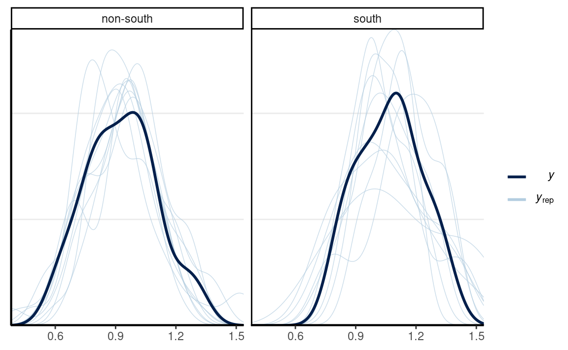
#> scale reduction factor on split chains (at convergence, Rhat = 1).Posterior predictive checks
# Check density (normality)
pp_check(m1, type = "dens_overlay_grouped", group = "South")
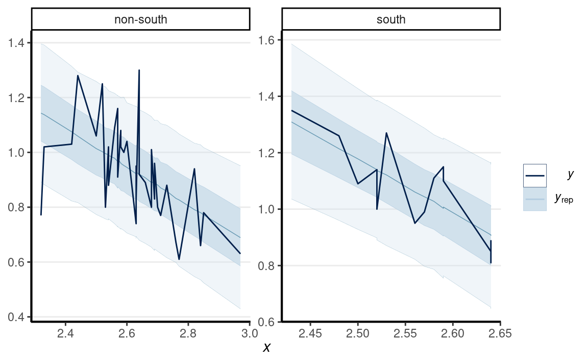
# Check prediction (a few outliers)
pp_check(m1,
    type = "ribbon_grouped", x = "MedianAgeMarriage",
    group = "South"
)
# Check errors (no clear pattern)
pp_check(m1,
    type = "error_scatter_avg_vs_x", x = "MedianAgeMarriage"
)

Conditional effects/simple slopes
Slope of MedianAgeMarriage when South = 0: \(\beta_1\)
Slope of MedianAgeMarriage when South = 1: \(\beta_1 + \beta_3\)
as_draws(m1) %>%
    mutate_variables(
        b_nonsouth = b_MedianAgeMarriage,
        b_south = b_MedianAgeMarriage + `b_Southsouth:MedianAgeMarriage`
    ) %>%
    posterior::subset_draws(
        variable = c("b_nonsouth", "b_south")
    ) %>%
    summarize_draws()
#> # A tibble: 2 × 10
#>   variable     mean median    sd   mad     q5    q95  rhat ess_bulk
#>   <chr>       <dbl>  <dbl> <dbl> <dbl>  <dbl>  <dbl> <dbl>    <dbl>
#> 1 b_nonsouth -0.699 -0.699 0.173 0.174 -0.983 -0.412  1.00    5161.
#> 2 b_south    -1.92  -1.93  0.598 0.581 -2.92  -0.937  1.00    3152.
#> # … with 1 more variable: ess_tail <dbl>plot(
conditional_effects(m1,
effects = "MedianAgeMarriage",
conditions = data.frame(South = c("south", "non-south"),
cond__ = c("South", "Non-South"))
),
points = TRUE
)

Interaction of Continuous Predictors
plotly::plot_ly(waffle_divorce,
                x = ~Marriage,
                y = ~MedianAgeMarriage,
                z = ~Divorce)
\[ \begin{aligned} D_i & \sim N(\mu_i, \sigma) \\ \mu_i & = \beta_0 + \beta_1 M_i + \beta_2 A_i + \beta_3 M_i \times A_i \\ \end{aligned} \]
# Use default priors (just for convenience here)
m2 <- brm(Divorce ~ Marriage * MedianAgeMarriage,
    data = waffle_divorce,
    seed = 941,
    iter = 4000
)
Centering
In the previous model, \(\beta_1\) is the slope of M → D when A is 0 (i.e., median marriage age = 0), and \(\beta_2\) is the slope of A → D when M is 0 (i.e., marriage rate is 0). These two are not very meaningful. Therefore, it is common to make the zero values more meaningful by doing centering.
Here, I use M - 2 as the predictor, so the zero point means a marriage rate of 2 per 10 adults; I use A - 2.5 as the other predictor, so the zero point means a median marriage rate of 25 years old.
\[\mu_i = \beta_0 + \beta_1 (M_i - 2) + \beta_2 (A_i - 2.5) + \beta_3 (M_i - 2) \times (A_i - 2.5)\]
msummary(list(`No centering` = m2, `centered` = m2c),
         estimate = "{estimate} [{conf.low}, {conf.high}]",
         statistic = NULL, fmt = 2)
| No centering | centered | |
|---|---|---|
| b_Intercept | 7.38 [2.95, 11.39] | 1.10 [1.03, 1.17] |
| b_Marriage | −1.97 [−3.92, 0.10] | |
| b_MedianAgeMarriage | −2.45 [−4.04, −0.79] | |
| b_Marriage × MedianAgeMarriage | 0.75 [−0.05, 1.54] | |
| sigma | 0.15 [0.12, 0.18] | 0.15 [0.12, 0.18] |
| b_IMarriageM2 | −0.08 [−0.24, 0.09] | |
| b_IMedianAgeMarriageM2.5 | −0.95 [−1.47, −0.47] | |
| b_IMarriageM2 × IMedianAgeMarriageM2.5 | 0.76 [−0.05, 1.62] | |
| Num.Obs. | 50 | 50 |
| ELPD | 21.4 | 21.1 |
| ELPD s.e. | 6.1 | 6.2 |
| LOOIC | −42.9 | −42.3 |
| LOOIC s.e. | 12.1 | 12.5 |
| WAIC | −43.3 | −43.1 |
| RMSE | 0.14 | 0.14 |
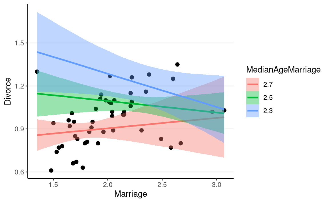
As shown in the table above, while the two models are equivalent in fit and give the same posterior distribution for \(\beta_3\), they differ in \(\beta_0\), \(\beta_1\), and \(\beta_2\).
plot(
    conditional_effects(m2c,
        effects = "Marriage:MedianAgeMarriage",
        int_conditions = list(MedianAgeMarriage = c(2.3, 2.5, 2.7)),
    ),
    points = TRUE
)
Multilevel Model
When data are naturally clustered in three or more segments or clusters, we can model interactions with a technique we have learned—hierarchical model with partial pooling. The difference is that we can have multiple parameters in each cluster. For example, consider the UC Berkeley admission data.
ggplot(berkeley_admit, aes(x = Gender)) +
    geom_pointrange(
        data = berkeley_admit %>%
            group_by(Gender) %>%
            summarise(
                padmit = sum(Admit) / sum(App),
                padmit_se = sqrt(padmit * (1 - padmit) / sum(App))
            ),
        aes(
            y = padmit,
            ymin = padmit - padmit_se, ymax = padmit + padmit_se
        )
    ) +
    labs(y = "Aggregated proportion admitted")

If we consider one department, we can model the number of admitted students for each gender as
\[ \begin{aligned} z_i & \sim \text{Bin}(N, \mu_i) \\ \mathrm{logit}(\mu_i) & = \eta_i \\ \eta_i & = \beta_0 + \beta_1 \text{Gender}_i \end{aligned} \]
So there are two coefficients, \(\beta_0\) and \(\beta_1\). We can then do the same for each of the six departments, and use partial pooling to pool the \(\beta_0\)’s into a common normal distribution, and the \(\beta_1\)’s into another common normal distribution. We can use \(j\) = 1, 2, \(\ldots\), \(J\) to index department, and then we have the following multilevel model:
\[ \begin{aligned} z_{ij} & \sim \text{Bin}(N_j, \mu_{ij}) \\ \mathrm{logit}(\mu_{ij}) & = \eta_{ij} \\ \eta_{ij} & = \beta_{0j} + \beta_{1j} \text{Gender}_{ij} \end{aligned}, \]
and use a multivariate normal distribution to partially pool the \(\beta_0\) and \(\beta_1\) coefficients. The multivariate normal allows the \(\beta_0\)’s and \(\beta_1\)’s to be correlated:
\[\begin{bmatrix} \beta_{0j} \\ \beta_{1j} \\ \end{bmatrix} \sim N_2\left( \begin{bmatrix} \gamma_0 \\ \gamma_1 \\ \end{bmatrix}, \mathbf{T} \right)\]
\(N_2(\cdot)\) means a bivariate normal distribution, and \(\mathbf{T}\) is a 2 \(\times\) 2 covariance matrix for \(\beta_0\) and \(\beta_1\). To set priors for \(\mathbf{T}\), we further decompose it into the standard deviations and the correlation matrix:
\[\mathbf{T} = \begin{bmatrix} \tau_0 & 0 \\ 0 & \tau_1 \\ \end{bmatrix} \begin{bmatrix} 1 & \\ \rho_{10} & 1 \\ \end{bmatrix} \begin{bmatrix} \tau_0 & 0 \\ 0 & \tau_1 \\ \end{bmatrix}\]
We can use the same inverse-gamma or half-\(t\) distributions for the \(\tau\)’s, as we’ve done in previous weeks. For \(\rho\), we need to introduce a new distribution: the LKJ distribution.
LKJ Prior
The LKJ Prior is a probability distribution for correlation matrices. A correlation matrix has 1 on all the diagonal elements. For example, a 2 \(\times\) 2 correlation matrix is
\[\begin{bmatrix} 1 & \\ 0.35 & 1 \end{bmatrix}\]
where the correlation is 0.35. Therefore, with two variables, there is one correlation; with three or more variables, the number of correlations will be \(q (q - 1) / 2\), where \(q\) is the number of variables.
For a correlation matrix of a given size, the LKJ prior has one shape parameter, \(\eta\), where \(\eta = 1\) corresponds to a uniform distribution of the correlations such that any correlations are equally likely, \(\eta \geq 1\) favors a matrix closer to an identity matrix so that the correlations are closer to zero, and \(\eta \leq 1\) favors a matrix with larger correlations. For a 2 \(\times\) 2 matrix, the distribution of the correlation, \(\rho\), with different \(\eta\) values are shown in the graph below:
dlkjcorr2 <- function(rho, eta = 1, log = FALSE) {
    # Function to compute the LKJ density given a correlation
    out <- (eta - 1) * log(1 - rho^2) -
        1 / 2 * log(pi) - lgamma(eta) + lgamma(eta + 1 / 2)
    if (!log) out <- exp(out)
    out
}
ggplot(tibble(rho = c(-1, 1)), aes(x = rho)) +
    stat_function(
        fun = dlkjcorr2, args = list(eta = 0.1),
        aes(col = "0.1"), n = 501
    ) +
    stat_function(
        fun = dlkjcorr2, args = list(eta = 0.5),
        aes(col = "0.5"), n = 501
    ) +
    stat_function(
        fun = dlkjcorr2, args = list(eta = 1),
        aes(col = "1"), n = 501
    ) +
    stat_function(
        fun = dlkjcorr2, args = list(eta = 2),
        aes(col = "2"), n = 501
    ) +
    stat_function(
        fun = dlkjcorr2, args = list(eta = 10),
        aes(col = "10"), n = 501
    ) +
    stat_function(
        fun = dlkjcorr2, args = list(eta = 100),
        aes(col = "100"), n = 501
    ) +
    labs(col = expression(eta), x = expression(rho), y = "Density")
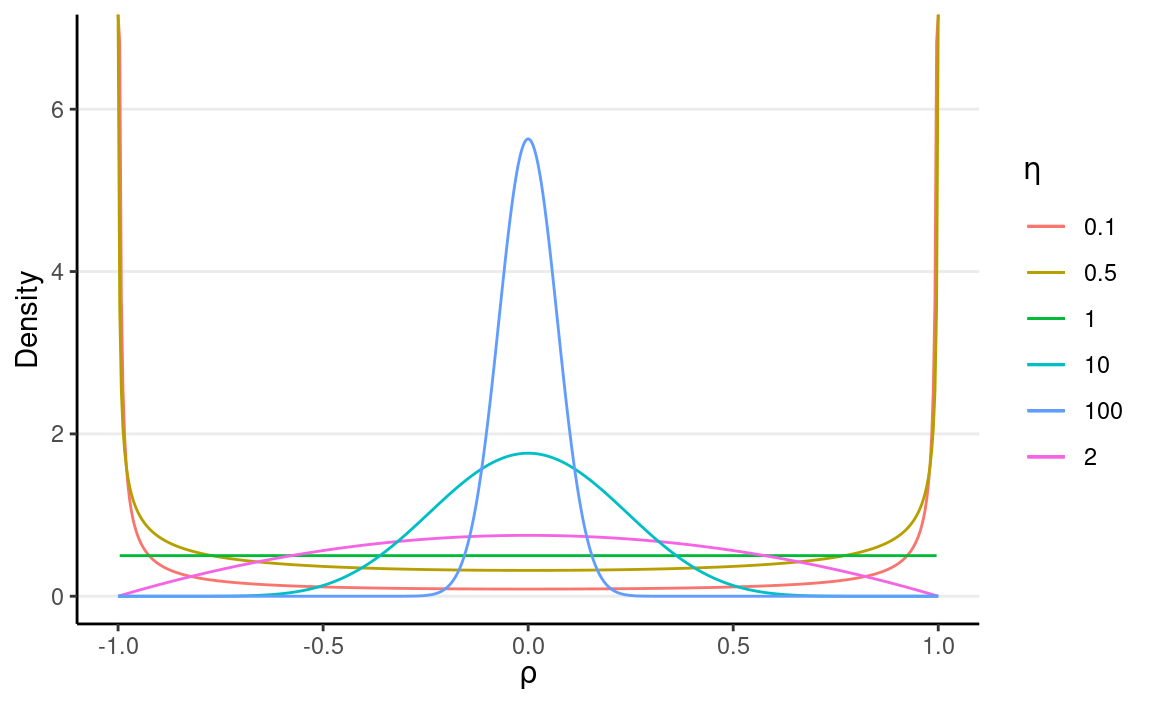
As you can see, when \(\eta\) increases, the correlation is more concentrated to zero.
The default in brms is to use \(\eta\) = 1, which is non-informative. If
you have a weak but informative belief that the correlations shouldn’t
be very large, using \(\eta\) = 2 is
reasonable.
Adding Cluster Means
In the multilevel modeling tradition, it is common also to include
the cluster means of the within-cluster predictors. In
this example, it means including the proportion of female applicants,
pFemale. So the equation becomes
\[\eta_{ij} = \beta_{0j} + \beta_{1j} \text{Gender}_{ij} + \gamma_2 \text{pFemale}_j,\]
with one additional \(\gamma_2\) coefficient (no \(j\) subscript).
# Obtain mean gender ratio at department level
berkeley_admit <- berkeley_admit %>%
    group_by(Dept) %>%
    mutate(pFemale = App[2] / sum(App)) %>%
    ungroup()
knitr::kable(berkeley_admit)
| Gender | Dept | Admit | App | pFemale |
|---|---|---|---|---|
| Male | A | 512 | 825 | 0.1157556 |
| Female | A | 89 | 108 | 0.1157556 |
| Male | B | 353 | 560 | 0.0427350 |
| Female | B | 17 | 25 | 0.0427350 |
| Male | C | 120 | 325 | 0.6459695 |
| Female | C | 202 | 593 | 0.6459695 |
| Male | D | 138 | 417 | 0.4734848 |
| Female | D | 131 | 375 | 0.4734848 |
| Male | E | 53 | 191 | 0.6729452 |
| Female | E | 94 | 393 | 0.6729452 |
| Male | F | 22 | 373 | 0.4775910 |
| Female | F | 24 | 341 | 0.4775910 |
Fitting the multilevel
model in brms
For this example, I’ll use these priors:
\[ \begin{aligned} \gamma_0 & \sim t_4(0, 5) \\ \gamma_1 & \sim t_4(0, 2.5) \\ \gamma_2 & \sim t_4(0, 5) \\ \tau_0 & \sim t^+_4(0, 3) \\ \tau_1 & \sim t^+_4(0, 3) \\ \rho & \sim \mathrm{LKJ}(2) \\ \end{aligned}, \]
m3 <- brm(Admit | trials(App) ~ Gender + pFemale + (Gender | Dept),
    data = berkeley_admit,
    family = binomial("logit"),
    prior = prior(student_t(4, 0, 5), class = "Intercept") +
        prior(student_t(4, 0, 2.5), class = "b", coef = "GenderFemale") +
        prior(student_t(4, 0, 5), class = "sd") +
        prior(lkj(2), class = "cor"),
    seed = 1547,
    iter = 4000,
    # a larger adapt_delta usually needed for MLM
    control = list(adapt_delta = .99, max_treedepth = 12)
)
The estimated \(\beta_0\) and \(\beta_1\) for each department is
coef(m3) # department-specific coefficients
#> $Dept
#> , , Intercept
#>
#> Estimate Est.Error Q2.5 Q97.5
#> A 0.8435257 0.4068035 0.02508813 1.681327
#> B 0.6560829 0.1741873 0.30299513 1.002269
#> C 1.2838795 2.2251880 -3.28413328 5.901322
#> D 0.6452240 1.6318918 -2.71918801 4.041556
#> E 0.9149422 2.3185424 -3.86584186 5.693197
#> F -1.3642409 1.6307569 -4.75616646 1.936458
#>
#> , , GenderFemale
#>
#> Estimate Est.Error Q2.5 Q97.5
#> A 0.82483971 0.2761378 0.2760824 1.3718327
#> B 0.25341066 0.3442156 -0.4185388 0.9582454
#> C -0.08142035 0.1353693 -0.3459999 0.1837492
#> D 0.09441718 0.1420221 -0.1868562 0.3696995
#> E -0.12284653 0.1888107 -0.4999416 0.2357683
#> F 0.14464805 0.2746741 -0.3910050 0.6838107
#>
#> , , pFemale
#>
#> Estimate Est.Error Q2.5 Q97.5
#> A -2.86759 3.440384 -10.04649 4.196067
#> B -2.86759 3.440384 -10.04649 4.196067
#> C -2.86759 3.440384 -10.04649 4.196067
#> D -2.86759 3.440384 -10.04649 4.196067
#> E -2.86759 3.440384 -10.04649 4.196067
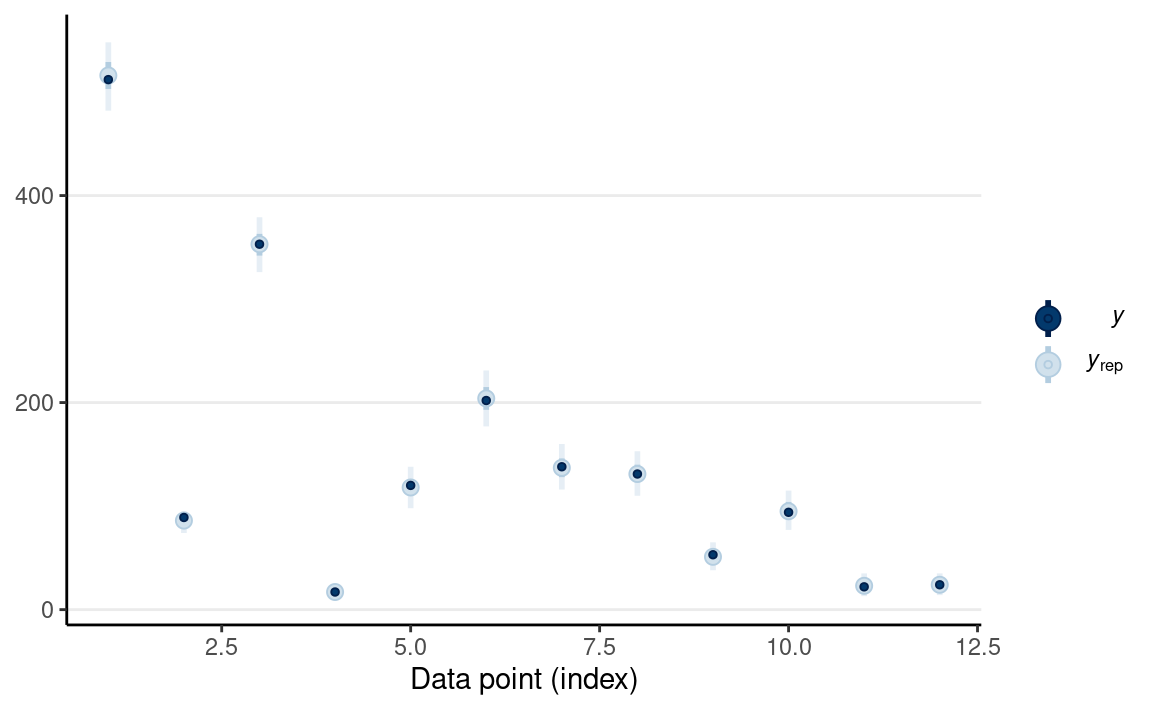
#> F -2.86759 3.440384 -10.04649 4.196067And a posterior predictive check
pp_check(m3, type = "intervals")
The plot below shows the predicted admission rate:
berkeley_admit %>%
    bind_cols(fitted(m3)) %>%
    ggplot(aes(x = Dept, y = Admit / App,
               col = Gender)) +
    geom_errorbar(aes(ymin = `Q2.5` / App, ymax = `Q97.5` / App),
    position = position_dodge(0.3), width = 0.2) +
    geom_point(position = position_dodge(width = 0.3)) +
    labs(y = "Posterior predicted acceptance rate")

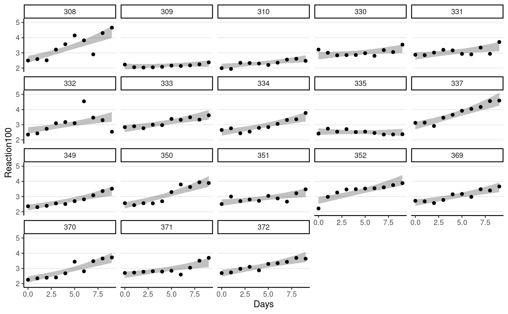
Bonus: Growth Model
- Data: Reaction times in a sleep deprivation study
- Predictor: Number of days of sleep deprivation
- Outcome: Daily average reaction time (ms)
- Cluster: 18 individuals (10 observations each)
\[ \begin{aligned} \text{Repeated-measure level:} \\ \text{Reaction10}_{ij} & \sim \mathrm{lognormal}(\mu_{ij}, \sigma) \\ \mu_{ij} & = \beta_{0j} + \beta_{1j} \text{Days}_{ij} \\ \text{Person level:} \\ \begin{bmatrix} \beta_{0j} \\ \beta_{1j} \\ \end{bmatrix} & \sim N_2\left( \begin{bmatrix} \gamma_0 \\ \gamma_1 \\ \end{bmatrix}, \mathbf{T} \right) \\ \mathbf{T} T & = \mathrm{diag}(\boldsymbol{\tau}) \boldsymbol{\Omega} \mathrm{diag}(\boldsymbol{\tau}) \\ \text{Priors:} \\ \gamma_0 & \sim N(0, 2) \\ \gamma_1 & \sim N(0, 1) \\ \tau_0, \tau_1 & \sim t^+_4(0, 2.5) \\ \boldsymbol{\Omega} & \sim \mathrm{LKJ}(2) \\ \sigma & \sim t^+_4(0, 2.5) \end{aligned} \]
m4 <- brm(
    Reaction100 ~ Days + (Days | Subject),
    data = sleepstudy,
    family = lognormal(),
    prior = c( # for intercept
        prior(normal(0, 2), class = "Intercept"),
        # for slope
        prior(std_normal(), class = "b"),
        # for tau0 and tau1
        prior(student_t(4, 0, 2.5), class = "sd"),
        # for correlation
        prior(lkj(2), class = "cor"),
        # for sigma
        prior(student_t(4, 0, 2.5), class = "sigma")
    ),
    control = list(adapt_delta = .95),
    seed = 2107,
    iter = 4000
)
m4
#>  Family: lognormal
#>   Links: mu = identity; sigma = identity
#> Formula: Reaction100 ~ Days + (Days | Subject)
#>    Data: sleepstudy (Number of observations: 180)
#>   Draws: 4 chains, each with iter = 4000; warmup = 2000; thin = 1;
#>          total post-warmup draws = 8000
#>
#> Group-Level Effects:
#> ~Subject (Number of levels: 18)
#>                     Estimate Est.Error l-95% CI u-95% CI Rhat
#> sd(Intercept)           0.12      0.03     0.07     0.18 1.00
#> sd(Days)                0.02      0.00     0.01     0.03 1.00
#> cor(Intercept,Days)    -0.02      0.26    -0.51     0.49 1.00
#>                     Bulk_ESS Tail_ESS
#> sd(Intercept)           3591     4533
#> sd(Days)                3489     4923
#> cor(Intercept,Days)     2938     4135
#>
#> Population-Level Effects:
#>           Estimate Est.Error l-95% CI u-95% CI Rhat Bulk_ESS Tail_ESS
#> Intercept     0.92      0.03     0.86     0.99 1.00     3282     4921
#> Days          0.03      0.01     0.02     0.04 1.00     4103     4832
#>
#> Family Specific Parameters:
#>       Estimate Est.Error l-95% CI u-95% CI Rhat Bulk_ESS Tail_ESS
#> sigma     0.08      0.00     0.07     0.09 1.00     7678     6095
#>
#> Draws were sampled using sampling(NUTS). For each parameter, Bulk_ESS
#> and Tail_ESS are effective sample size measures, and Rhat is the potential
#> scale reduction factor on split chains (at convergence, Rhat = 1).
Model estimate: the shaded band is the predicted mean trajectory
sleepstudy %>%
    bind_cols(fitted(m4)) %>%
    ggplot(aes(x = Days, y = Reaction100)) +
    geom_ribbon(aes(y = Estimate, ymin = `Q2.5`,
                    ymax = `Q97.5`), alpha = 0.3) +
    geom_point() +
    facet_wrap(~ Subject)
Last updated
#> [1] "April 21, 2022"