Poisson Model

Please note: This document uses count data on fatal police shootings.

library(psych)
library(tidyverse)
library(bayesplot)
library(posterior)
theme_set(theme_classic() +
    theme(panel.grid.major.y = element_line(color = "grey92")))

I came across this data set from https://andrewpwheeler.com/2021/01/11/checking-a-poisson-distribution-fit-an-example-with-officer-involved-shooting-deaths-wapo-data-r-functions/

As explained here, the data are by the Washington Post in an effort to record every fatal shooting in the United States by a police officer since January 1, 2015.

Research Question

What’s the rate of fatal police shootings in the United States per year?

Data Import and Pre-Processing

# Import data
fps_dat <- read_csv(
    "https://raw.githubusercontent.com/washingtonpost/data-police-shootings/master/fatal-police-shootings-data.csv"
)

We first count the data by year

# Create a year column
fps_dat <- fps_dat %>%
    mutate(year = format(date, format = "%Y"))
# Filter out 2022
fps_1521 <- filter(fps_dat, year != "2022")
count(fps_1521, year)

#> # A tibble: 7 × 2
#>   year      n
#>   <chr> <int>
#> 1 2015    994
#> 2 2016    958
#> 3 2017    981
#> 4 2018    985
#> 5 2019    999
#> 6 2020   1020
#> 7 2021   1054

Poisson Model

Our interest is the rate of occurrence of fatal police shootings per year. Denote this as \(\theta\). The support of \(\theta\) is \([0, \infty)\).

A Poisson model is usually a starting point for analyzing count data in a fixed amount of time. It assumes that the data follow a Poisson distribution with a fixed rate parameter: \[P(y \mid \theta) \propto \theta^y \exp(- \theta),\] where the data can be any non-negative integers (no decimals).

Choosing a Prior

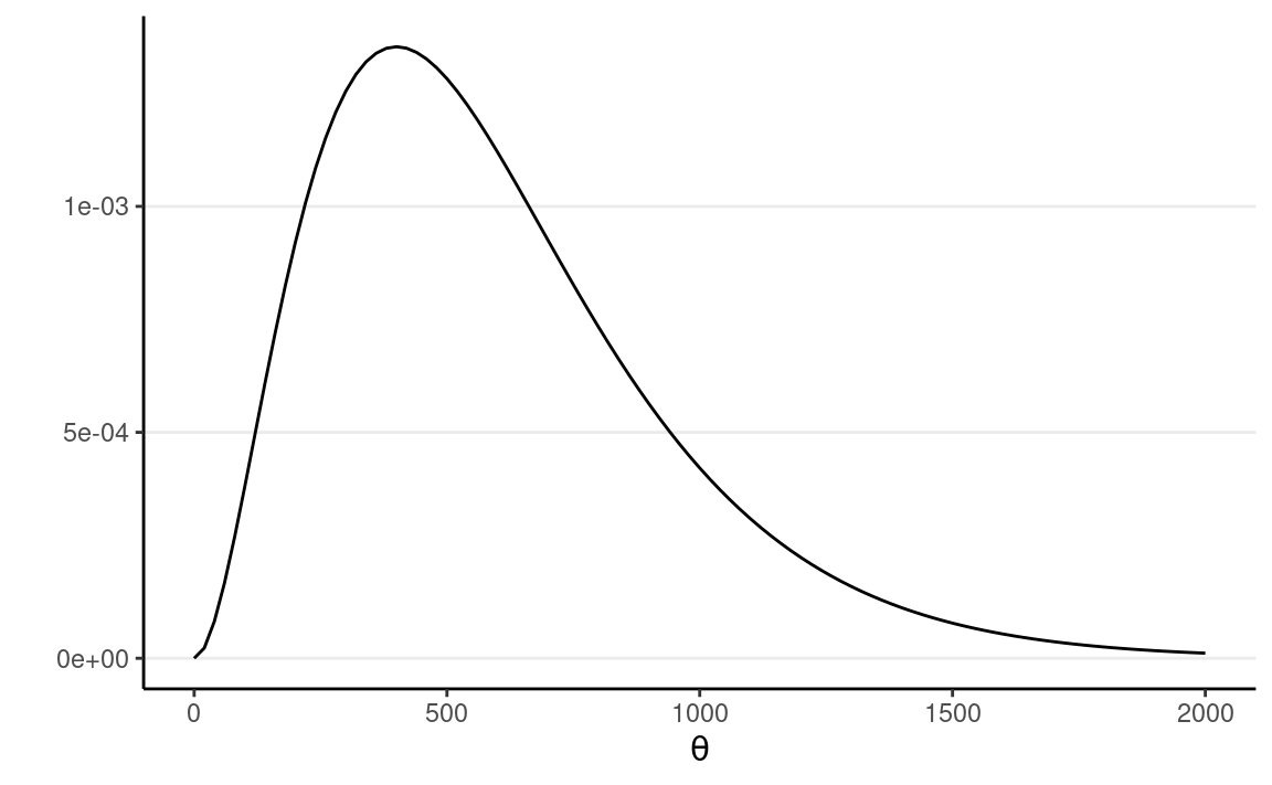
The Gamma distribution has support: \([0, \infty)\), and is a conjugate family to the Poisson model. The Gamma distribution has the form \[P(\theta) \propto \theta^{a - 1} \exp(-b \theta),\] where \(a\) is the prior incidence rate, and \(b\) is the number of prior data points to control for the prior strength. Here, without much prior knowledge, I would simply guess there is one fatal shooting per state per month, so 600 shootings per year, but my belief is pretty weak, so I will assume a prior \(b\) of 1 / 200 (one observation is one year). The \(a\) will be 600 * \(b\) = 3.

Here’s a plot:

ggplot(tibble(th = c(0, 2000)), aes(x = th)) +
    stat_function(fun = dgamma,
    args = list(shape = 3, rate = 1 / 200)) +
    labs(y = "", x = expression(theta))

Prior predictive check

set.seed(2200)
num_draws <- 100
sim_theta <- rgamma(num_draws, shape = 3, rate = 1 / 200)
# Initialize a time-series plot
ts_plot <- ggplot(count(fps_1521, year), aes(x = year, y = n))
# Simulate time series from the prior, and add to plot
# Initialize an S by N matrix to store the simulated data
y_tilde <- matrix(NA,
                  nrow = length(sim_theta),
                  ncol = 7)
colnames(y_tilde) <- 2015:2021  # add column names
for (s in seq_along(sim_theta)) {
    theta_s <- sim_theta[s]
    y_tilde[s,] <- rpois(7, lambda = theta_s)
}
# Convert to a data frame
y_tilde_df <- as_tibble(y_tilde) %>%
    rownames_to_column(var = "id") %>%
    pivot_longer(
        cols = -id,
        names_to = "year",
        values_to = "y_tilde"
    )
ts_plot +
    geom_line(
        data = y_tilde_df,
        aes(y = y_tilde, group = id),
        alpha = 0.3,
        col = "skyblue"
    ) +
    # add observed data
    geom_point() +
    geom_line(aes(group = 1))

Posterior

With a conjugate prior, the posterior distribution is Gamma(\(a\) + \(\sum_{i = 1}^N y_i\), \(b\) + \(N\)).

ggplot(tibble(th = c(0, 2000)), aes(x = th)) +
    stat_function(fun = dgamma,
    args = list(shape = 3 + nrow(fps_1521),
                rate = 1 / 200 + 7), n = 501) +
    labs(y = "", x = expression(theta))

Summary

Use simulation

num_draws <- 1000
post_theta <- rgamma(num_draws, shape = 3 + nrow(fps_1521),
                    rate = 1 / 200 + 7)
# Use the `posterior` package
posterior::as_draws(tibble(theta = post_theta)) %>%
    summarize_draws()

#> # A tibble: 1 × 10
#>   variable  mean median    sd   mad    q5   q95  rhat ess_bulk
#>   <chr>    <dbl>  <dbl> <dbl> <dbl> <dbl> <dbl> <dbl>    <dbl>
#> 1 theta     998.   998.  11.6  11.4  979. 1017.  1.00    1075.
#> # … with 1 more variable: ess_tail <dbl>

So the estimated rate is 987 per year, with a 90% CI [967, 1006].

Posterior Predictive Check

# Initialize a time-series plot
ts_plot <- ggplot(count(fps_1521, year), aes(x = year, y = n))
# Simulate time series from the prior, and add to plot
# Initialize an S by N matrix to store the simulated data
y_tilde <- matrix(NA,
                  nrow = length(post_theta),
                  ncol = 7)
colnames(y_tilde) <- 2015:2021  # add column names
for (s in seq_along(post_theta)) {
    theta_s <- post_theta[s]
    y_tilde[s,] <- rpois(7, lambda = theta_s)
}
# Convert to a data frame
y_tilde_df <- as_tibble(y_tilde) %>%
    rownames_to_column(var = "id") %>%
    pivot_longer(
        cols = -id,
        names_to = "year",
        values_to = "y_tilde"
    )
ts_plot +
    geom_line(
        data = y_tilde_df,
        aes(y = y_tilde, group = id),
        alpha = 0.2,
        col = "skyblue"
    ) +
    # add observed data
    geom_point() +
    geom_line(aes(group = 1))

Last updated

#> [1] "February 11, 2022"