library(tidyverse)
library(haven)  # for importing SPSS data
library(here)
library(rstan)
rstan_options(auto_write = TRUE)  # save compiled STAN object
library(posterior)  # for summarizing draws
library(bayesplot)  # for plotting
theme_set(theme_classic() +
    theme(panel.grid.major.y = element_line(color = "grey92")))
Data
We will use the data in Frank, Biberci, and Verschuere (2019), which is a replication study examining the response time (RT) when lying. Specifically, the researchers were interested in whether RT is shorter or longer when lying in the native language. In the original study, the researchers found that the difference between telling a lie and a truth (lie-truth difference) was smaller in English than in German for native German speakers. In the replication study, the same design was used to see whether the findings could be replicated on Dutch speakers. The data can be found at https://osf.io/x4rfk/.
Instead of looking at lie-truth difference across languages, we will start by comparing the difference in RT for telling a lie in Dutch between males (man) and females (vrouw), as the model is easier to understand for independent sample comparisons and can be applied generally for between-subject experimental designs.
datfile <- here("data_files", "ENDFILE.xlsx")
if (!file.exists(datfile)) {
    dir.create(here("data_files"))
    download.file("https://osf.io/gtjf6/download",
        destfile = datfile
    )
}
lies <- readxl::read_excel(datfile)
# Exclude missing values
lies_cc <- drop_na(lies, LDMRT)
# Rescale response time from ms to sec
lies_cc <- lies_cc %>%
# Use `across()` for doing the same operation on multiple variables
# `~ . / 1000` means apply the operation x / 1000 for each
# specified variable x
mutate(across(LDMRT:TEMRT, ~ . / 1000,
# create new variables by adding `_sec` to the new
# variable names
.names = "{.col}_sec"))
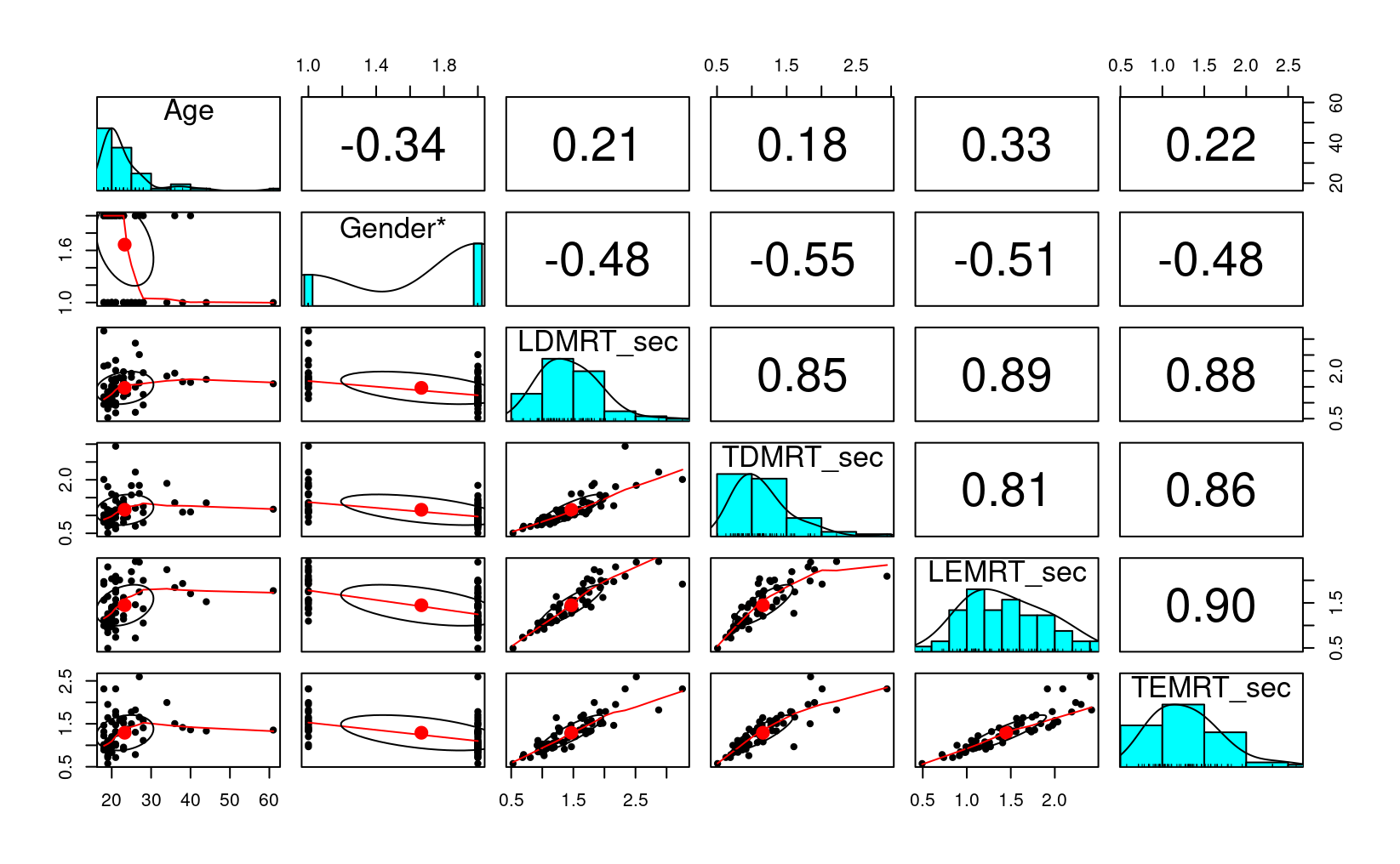
# Describe the data
psych::describe(lies_cc %>% select(Age, LDMRT_sec:TEMRT_sec))
#>           vars  n  mean   sd median trimmed  mad   min   max range
#> Age          1 63 23.29 7.32  21.00   21.69 2.97 18.00 61.00 43.00
#> LDMRT_sec    2 63  1.47 0.51   1.41    1.42 0.47  0.53  3.26  2.73
#> TDMRT_sec    3 63  1.16 0.43   1.09    1.10 0.35  0.51  2.94  2.43
#> LEMRT_sec    4 63  1.45 0.46   1.41    1.43 0.50  0.49  2.42  1.93
#> TEMRT_sec    5 63  1.29 0.41   1.28    1.26 0.42  0.57  2.60  2.02
#>           skew kurtosis   se
#> Age       2.91    10.21 0.92
#> LDMRT_sec 0.97     1.41 0.06
#> TDMRT_sec 1.54     3.27 0.05
#> LEMRT_sec 0.29    -0.80 0.06
#> TEMRT_sec 0.86     0.69 0.05
# Plot the data
lies_cc %>%
select(Age, Gender, LDMRT_sec:TEMRT_sec) %>%
psych::pairs.panels()
Plots
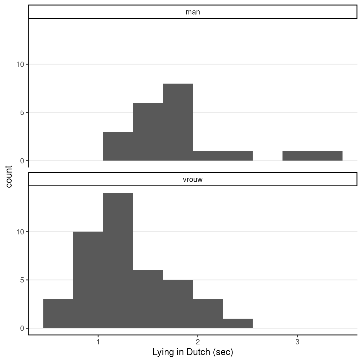
ggplot(lies_cc, aes(x = LDMRT_sec)) +
    geom_histogram(binwidth = 0.3) +
    facet_wrap(~ Gender,  ncol = 1) +
    labs(x = "Lying in Dutch (sec)")
Independent Sample \(t\)-Test
Frequentist
# Independent-sample t-test
t.test(LDMRT_sec ~ Gender, data = lies_cc)
#>
#>  Welch Two Sample t-test
#>
#> data:  LDMRT_sec by Gender
#> t = 4.011, df = 34.317, p-value = 0.00031
#> alternative hypothesis: true difference in means between group man and group vrouw is not equal to 0
#> 95 percent confidence interval:
#>  0.2548537 0.7779701
#> sample estimates:
#>   mean in group man mean in group vrouw
#>            1.811999            1.295587
Bayesian
The \(t\)-test above does not directly show the underlying model. In fully Bayesian analyses, this has to be made explicit. A statistical model states the underlying assumptions of the statistical procedure. And to say more directly, a model is mostly a set of distributional assumptions. Below is the model for a \(t\)-test:
\[ \begin{aligned} \text{RT}_{i, \text{male}} & \sim N(\mu_1, \sigma_1) \\ \text{RT}_{i, \text{female}} & \sim N(\mu_2, \sigma_2) \end{aligned} \]
Note that we don’t assume \(\sigma_1 = \sigma_2\), which correspond to the Welch’s \(t\) test. We could impose homogeneity of variance across groups using a common \(\sigma\).
# 1. form the data list for Stan
stan_dat <- with(lies_cc,
    list(N1 = sum(Gender == "man"),
         N2 = sum(Gender == "vrouw"),
         y1 = LDMRT_sec[which(Gender == "man")],
         y2 = LDMRT_sec[which(Gender == "vrouw")])
)
# 2. Run Stan (with lines for the likelihood commented out)
m0 <- stan(
    file = here("stan", "normal_2group.stan"),
    data = stan_dat,
    seed = 2151  # for reproducibility
)
#>
#> SAMPLING FOR MODEL 'normal_2group' NOW (CHAIN 1).
#> Chain 1:
#> Chain 1: Gradient evaluation took 8e-06 seconds
#> Chain 1: 1000 transitions using 10 leapfrog steps per transition would take 0.08 seconds.
#> Chain 1: Adjust your expectations accordingly!
#> Chain 1:
#> Chain 1:
#> Chain 1: Iteration:    1 / 2000 [  0%]  (Warmup)
#> Chain 1: Iteration:  200 / 2000 [ 10%]  (Warmup)
#> Chain 1: Iteration:  400 / 2000 [ 20%]  (Warmup)
#> Chain 1: Iteration:  600 / 2000 [ 30%]  (Warmup)
#> Chain 1: Iteration:  800 / 2000 [ 40%]  (Warmup)
#> Chain 1: Iteration: 1000 / 2000 [ 50%]  (Warmup)
#> Chain 1: Iteration: 1001 / 2000 [ 50%]  (Sampling)
#> Chain 1: Iteration: 1200 / 2000 [ 60%]  (Sampling)
#> Chain 1: Iteration: 1400 / 2000 [ 70%]  (Sampling)
#> Chain 1: Iteration: 1600 / 2000 [ 80%]  (Sampling)
#> Chain 1: Iteration: 1800 / 2000 [ 90%]  (Sampling)
#> Chain 1: Iteration: 2000 / 2000 [100%]  (Sampling)
#> Chain 1:
#> Chain 1:  Elapsed Time: 0.026117 seconds (Warm-up)
#> Chain 1:                0.024948 seconds (Sampling)
#> Chain 1:                0.051065 seconds (Total)
#> Chain 1:
#>
#> SAMPLING FOR MODEL 'normal_2group' NOW (CHAIN 2).
#> Chain 2:
#> Chain 2: Gradient evaluation took 1.1e-05 seconds
#> Chain 2: 1000 transitions using 10 leapfrog steps per transition would take 0.11 seconds.
#> Chain 2: Adjust your expectations accordingly!
#> Chain 2:
#> Chain 2:
#> Chain 2: Iteration:    1 / 2000 [  0%]  (Warmup)
#> Chain 2: Iteration:  200 / 2000 [ 10%]  (Warmup)
#> Chain 2: Iteration:  400 / 2000 [ 20%]  (Warmup)
#> Chain 2: Iteration:  600 / 2000 [ 30%]  (Warmup)
#> Chain 2: Iteration:  800 / 2000 [ 40%]  (Warmup)
#> Chain 2: Iteration: 1000 / 2000 [ 50%]  (Warmup)
#> Chain 2: Iteration: 1001 / 2000 [ 50%]  (Sampling)
#> Chain 2: Iteration: 1200 / 2000 [ 60%]  (Sampling)
#> Chain 2: Iteration: 1400 / 2000 [ 70%]  (Sampling)
#> Chain 2: Iteration: 1600 / 2000 [ 80%]  (Sampling)
#> Chain 2: Iteration: 1800 / 2000 [ 90%]  (Sampling)
#> Chain 2: Iteration: 2000 / 2000 [100%]  (Sampling)
#> Chain 2:
#> Chain 2:  Elapsed Time: 0.02734 seconds (Warm-up)
#> Chain 2:                0.027084 seconds (Sampling)
#> Chain 2:                0.054424 seconds (Total)
#> Chain 2:
#>
#> SAMPLING FOR MODEL 'normal_2group' NOW (CHAIN 3).
#> Chain 3:
#> Chain 3: Gradient evaluation took 6e-06 seconds
#> Chain 3: 1000 transitions using 10 leapfrog steps per transition would take 0.06 seconds.
#> Chain 3: Adjust your expectations accordingly!
#> Chain 3:
#> Chain 3:
#> Chain 3: Iteration:    1 / 2000 [  0%]  (Warmup)
#> Chain 3: Iteration:  200 / 2000 [ 10%]  (Warmup)
#> Chain 3: Iteration:  400 / 2000 [ 20%]  (Warmup)
#> Chain 3: Iteration:  600 / 2000 [ 30%]  (Warmup)
#> Chain 3: Iteration:  800 / 2000 [ 40%]  (Warmup)
#> Chain 3: Iteration: 1000 / 2000 [ 50%]  (Warmup)
#> Chain 3: Iteration: 1001 / 2000 [ 50%]  (Sampling)
#> Chain 3: Iteration: 1200 / 2000 [ 60%]  (Sampling)
#> Chain 3: Iteration: 1400 / 2000 [ 70%]  (Sampling)
#> Chain 3: Iteration: 1600 / 2000 [ 80%]  (Sampling)
#> Chain 3: Iteration: 1800 / 2000 [ 90%]  (Sampling)
#> Chain 3: Iteration: 2000 / 2000 [100%]  (Sampling)
#> Chain 3:
#> Chain 3:  Elapsed Time: 0.031023 seconds (Warm-up)
#> Chain 3:                0.026521 seconds (Sampling)
#> Chain 3:                0.057544 seconds (Total)
#> Chain 3:
#>
#> SAMPLING FOR MODEL 'normal_2group' NOW (CHAIN 4).
#> Chain 4:
#> Chain 4: Gradient evaluation took 8e-06 seconds
#> Chain 4: 1000 transitions using 10 leapfrog steps per transition would take 0.08 seconds.
#> Chain 4: Adjust your expectations accordingly!
#> Chain 4:
#> Chain 4:
#> Chain 4: Iteration:    1 / 2000 [  0%]  (Warmup)
#> Chain 4: Iteration:  200 / 2000 [ 10%]  (Warmup)
#> Chain 4: Iteration:  400 / 2000 [ 20%]  (Warmup)
#> Chain 4: Iteration:  600 / 2000 [ 30%]  (Warmup)
#> Chain 4: Iteration:  800 / 2000 [ 40%]  (Warmup)
#> Chain 4: Iteration: 1000 / 2000 [ 50%]  (Warmup)
#> Chain 4: Iteration: 1001 / 2000 [ 50%]  (Sampling)
#> Chain 4: Iteration: 1200 / 2000 [ 60%]  (Sampling)
#> Chain 4: Iteration: 1400 / 2000 [ 70%]  (Sampling)
#> Chain 4: Iteration: 1600 / 2000 [ 80%]  (Sampling)
#> Chain 4: Iteration: 1800 / 2000 [ 90%]  (Sampling)
#> Chain 4: Iteration: 2000 / 2000 [100%]  (Sampling)
#> Chain 4:
#> Chain 4:  Elapsed Time: 0.026595 seconds (Warm-up)
#> Chain 4:                0.027055 seconds (Sampling)
#> Chain 4:                0.05365 seconds (Total)
#> Chain 4:#> Inference for Stan model: normal_2group.
#> 4 chains, each with iter=2000; warmup=1000; thin=1;
#> post-warmup draws per chain=1000, total post-warmup draws=4000.
#>
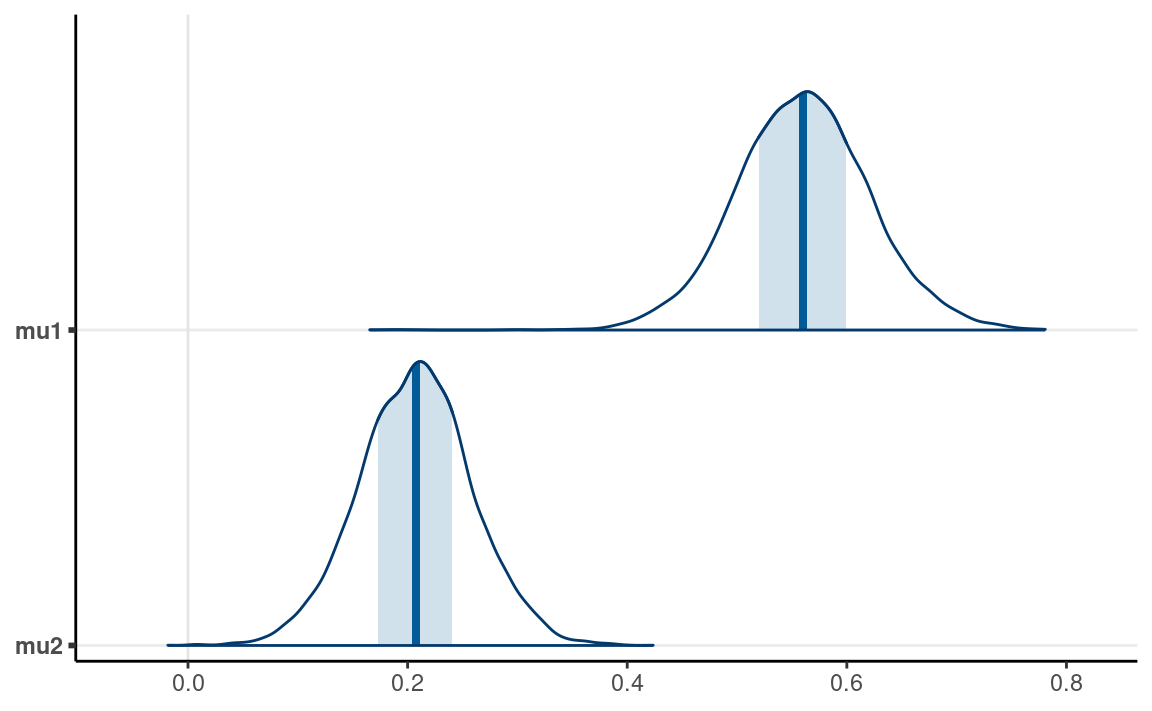
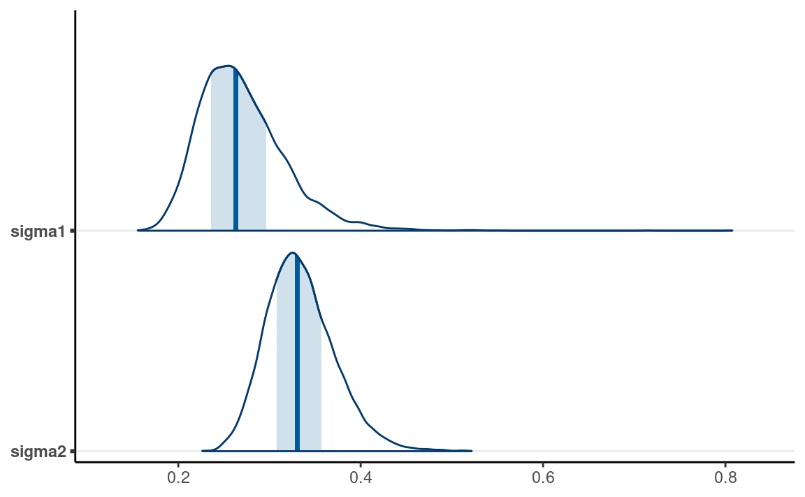
#> mean se_mean sd 2.5% 25% 50% 75% 97.5% n_eff Rhat
#> mu1 1.79 0 0.12 1.54 1.71 1.79 1.88 2.03 3643 1
#> mu2 1.29 0 0.07 1.16 1.25 1.29 1.34 1.42 3361 1
#> sigma1 0.54 0 0.09 0.40 0.47 0.53 0.59 0.75 3105 1
#> sigma2 0.44 0 0.05 0.36 0.40 0.43 0.47 0.54 4101 1
#>
#> Samples were drawn using NUTS(diag_e) at Thu Apr 28 11:39:18 2022.
#> For each parameter, n_eff is a crude measure of effective sample size,
#> and Rhat is the potential scale reduction factor on split chains (at
#> convergence, Rhat=1).Normal models are not robust
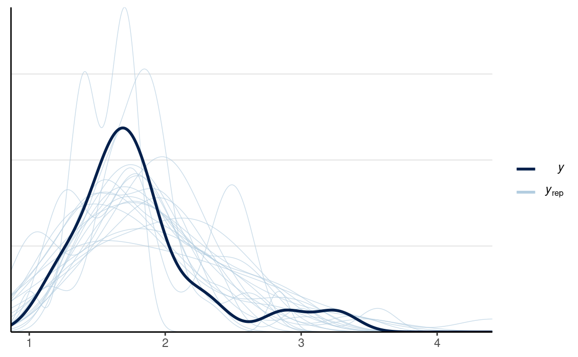
Let’s add one outlier to the vrouw group with a value of 8.
# 1. form the data list for Stan
out_dat <- with(lies_cc,
    list(N1 = sum(Gender == "man"),
         N2 = sum(Gender == "vrouw") + 1,
         y1 = LDMRT_sec[which(Gender == "man")],
         y2 = c(LDMRT_sec[which(Gender == "vrouw")], 8))
)
# 2. Run Stan (with lines for the likelihood commented out)
m0_out <- stan(
    file = here("stan", "normal_2group.stan"),
    data = out_dat,
    seed = 2151  # for reproducibility
)
#>
#> SAMPLING FOR MODEL 'normal_2group' NOW (CHAIN 1).
#> Chain 1:
#> Chain 1: Gradient evaluation took 8e-06 seconds
#> Chain 1: 1000 transitions using 10 leapfrog steps per transition would take 0.08 seconds.
#> Chain 1: Adjust your expectations accordingly!
#> Chain 1:
#> Chain 1:
#> Chain 1: Iteration:    1 / 2000 [  0%]  (Warmup)
#> Chain 1: Iteration:  200 / 2000 [ 10%]  (Warmup)
#> Chain 1: Iteration:  400 / 2000 [ 20%]  (Warmup)
#> Chain 1: Iteration:  600 / 2000 [ 30%]  (Warmup)
#> Chain 1: Iteration:  800 / 2000 [ 40%]  (Warmup)
#> Chain 1: Iteration: 1000 / 2000 [ 50%]  (Warmup)
#> Chain 1: Iteration: 1001 / 2000 [ 50%]  (Sampling)
#> Chain 1: Iteration: 1200 / 2000 [ 60%]  (Sampling)
#> Chain 1: Iteration: 1400 / 2000 [ 70%]  (Sampling)
#> Chain 1: Iteration: 1600 / 2000 [ 80%]  (Sampling)
#> Chain 1: Iteration: 1800 / 2000 [ 90%]  (Sampling)
#> Chain 1: Iteration: 2000 / 2000 [100%]  (Sampling)
#> Chain 1:
#> Chain 1:  Elapsed Time: 0.035051 seconds (Warm-up)
#> Chain 1:                0.033921 seconds (Sampling)
#> Chain 1:                0.068972 seconds (Total)
#> Chain 1:
#>
#> SAMPLING FOR MODEL 'normal_2group' NOW (CHAIN 2).
#> Chain 2:
#> Chain 2: Gradient evaluation took 8e-06 seconds
#> Chain 2: 1000 transitions using 10 leapfrog steps per transition would take 0.08 seconds.
#> Chain 2: Adjust your expectations accordingly!
#> Chain 2:
#> Chain 2:
#> Chain 2: Iteration:    1 / 2000 [  0%]  (Warmup)
#> Chain 2: Iteration:  200 / 2000 [ 10%]  (Warmup)
#> Chain 2: Iteration:  400 / 2000 [ 20%]  (Warmup)
#> Chain 2: Iteration:  600 / 2000 [ 30%]  (Warmup)
#> Chain 2: Iteration:  800 / 2000 [ 40%]  (Warmup)
#> Chain 2: Iteration: 1000 / 2000 [ 50%]  (Warmup)
#> Chain 2: Iteration: 1001 / 2000 [ 50%]  (Sampling)
#> Chain 2: Iteration: 1200 / 2000 [ 60%]  (Sampling)
#> Chain 2: Iteration: 1400 / 2000 [ 70%]  (Sampling)
#> Chain 2: Iteration: 1600 / 2000 [ 80%]  (Sampling)
#> Chain 2: Iteration: 1800 / 2000 [ 90%]  (Sampling)
#> Chain 2: Iteration: 2000 / 2000 [100%]  (Sampling)
#> Chain 2:
#> Chain 2:  Elapsed Time: 0.028427 seconds (Warm-up)
#> Chain 2:                0.028419 seconds (Sampling)
#> Chain 2:                0.056846 seconds (Total)
#> Chain 2:
#>
#> SAMPLING FOR MODEL 'normal_2group' NOW (CHAIN 3).
#> Chain 3:
#> Chain 3: Gradient evaluation took 8e-06 seconds
#> Chain 3: 1000 transitions using 10 leapfrog steps per transition would take 0.08 seconds.
#> Chain 3: Adjust your expectations accordingly!
#> Chain 3:
#> Chain 3:
#> Chain 3: Iteration:    1 / 2000 [  0%]  (Warmup)
#> Chain 3: Iteration:  200 / 2000 [ 10%]  (Warmup)
#> Chain 3: Iteration:  400 / 2000 [ 20%]  (Warmup)
#> Chain 3: Iteration:  600 / 2000 [ 30%]  (Warmup)
#> Chain 3: Iteration:  800 / 2000 [ 40%]  (Warmup)
#> Chain 3: Iteration: 1000 / 2000 [ 50%]  (Warmup)
#> Chain 3: Iteration: 1001 / 2000 [ 50%]  (Sampling)
#> Chain 3: Iteration: 1200 / 2000 [ 60%]  (Sampling)
#> Chain 3: Iteration: 1400 / 2000 [ 70%]  (Sampling)
#> Chain 3: Iteration: 1600 / 2000 [ 80%]  (Sampling)
#> Chain 3: Iteration: 1800 / 2000 [ 90%]  (Sampling)
#> Chain 3: Iteration: 2000 / 2000 [100%]  (Sampling)
#> Chain 3:
#> Chain 3:  Elapsed Time: 0.027191 seconds (Warm-up)
#> Chain 3:                0.02895 seconds (Sampling)
#> Chain 3:                0.056141 seconds (Total)
#> Chain 3:
#>
#> SAMPLING FOR MODEL 'normal_2group' NOW (CHAIN 4).
#> Chain 4:
#> Chain 4: Gradient evaluation took 6e-06 seconds
#> Chain 4: 1000 transitions using 10 leapfrog steps per transition would take 0.06 seconds.
#> Chain 4: Adjust your expectations accordingly!
#> Chain 4:
#> Chain 4:
#> Chain 4: Iteration:    1 / 2000 [  0%]  (Warmup)
#> Chain 4: Iteration:  200 / 2000 [ 10%]  (Warmup)
#> Chain 4: Iteration:  400 / 2000 [ 20%]  (Warmup)
#> Chain 4: Iteration:  600 / 2000 [ 30%]  (Warmup)
#> Chain 4: Iteration:  800 / 2000 [ 40%]  (Warmup)
#> Chain 4: Iteration: 1000 / 2000 [ 50%]  (Warmup)
#> Chain 4: Iteration: 1001 / 2000 [ 50%]  (Sampling)
#> Chain 4: Iteration: 1200 / 2000 [ 60%]  (Sampling)
#> Chain 4: Iteration: 1400 / 2000 [ 70%]  (Sampling)
#> Chain 4: Iteration: 1600 / 2000 [ 80%]  (Sampling)
#> Chain 4: Iteration: 1800 / 2000 [ 90%]  (Sampling)
#> Chain 4: Iteration: 2000 / 2000 [100%]  (Sampling)
#> Chain 4:
#> Chain 4:  Elapsed Time: 0.037111 seconds (Warm-up)
#> Chain 4:                0.032667 seconds (Sampling)
#> Chain 4:                0.069778 seconds (Total)
#> Chain 4:#> Inference for Stan model: normal_2group.
#> 4 chains, each with iter=2000; warmup=1000; thin=1;
#> post-warmup draws per chain=1000, total post-warmup draws=4000.
#>
#> mean se_mean sd 2.5% 25% 50% 75% 97.5% n_eff Rhat
#> mu1 1.79 0 0.11 1.56 1.72 1.80 1.87 2.01 3267 1
#> mu2 1.43 0 0.17 1.11 1.32 1.43 1.54 1.75 4525 1
#> sigma1 0.54 0 0.09 0.39 0.47 0.53 0.59 0.75 3447 1
#> sigma2 1.11 0 0.12 0.90 1.03 1.10 1.19 1.38 3953 1
#>
#> Samples were drawn using NUTS(diag_e) at Thu Apr 28 11:39:20 2022.
#> For each parameter, n_eff is a crude measure of effective sample size,
#> and Rhat is the potential scale reduction factor on split chains (at
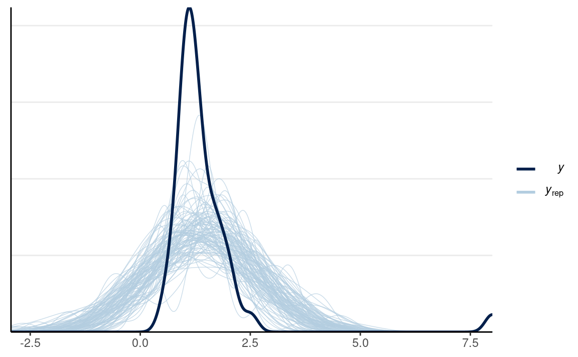
#> convergence, Rhat=1).# PPC for Group 2 (vrouw)
y2_tilde <- extract(m0_out, pars = "y2_rep")$y2_rep
# Randomly sample 100 data sets (to make plotting faster)
set.seed(2154)
selected_rows <- sample.int(nrow(y2_tilde), size = 100)
ppc_dens_overlay(out_dat$y2,
yrep = y2_tilde[selected_rows, ],
bw = "SJ")
Bayesian Robust Model
One robust option against (some) outliers is the \(t\) model. While fitting a \(t\) model is more challenging in frequentist analyses, in Bayesian, it is as easy as the normal model. Specifically,
\[ \begin{aligned} \text{RT}_{i, \text{male}} & \sim t_\nu(\mu_1, \sigma_1) \\ \text{RT}_{i, \text{female}} & \sim t_\nu(\mu_2, \sigma_2), \end{aligned} \]
where \(\nu \in [1, \infty)\) is the degrees of freedom parameter, also called the normality parameter. The larger \(\nu\), the more normal the distribution is. On the other hand, when \(\nu\) is close to 1, the distribution allows for highly extreme values. When \(\nu = 1\), the distribution is from a Cauchy family. The only difference from a normal model is that we need to assign a prior for \(\nu\). A good option is Gamma(2, 0.1) (see https://github.com/stan-dev/stan/wiki/Prior-Choice-Recommendations#prior-for-degrees-of-freedom-in-students-t-distribution).
# 2. Run Stan (with lines for the likelihood commented out)
m0r <- stan(
    file = here("stan", "robust_2group.stan"),
    data = out_dat,
    seed = 2151  # for reproducibility
)
#>
#> SAMPLING FOR MODEL 'robust_2group' NOW (CHAIN 1).
#> Chain 1:
#> Chain 1: Gradient evaluation took 1.4e-05 seconds
#> Chain 1: 1000 transitions using 10 leapfrog steps per transition would take 0.14 seconds.
#> Chain 1: Adjust your expectations accordingly!
#> Chain 1:
#> Chain 1:
#> Chain 1: Iteration:    1 / 2000 [  0%]  (Warmup)
#> Chain 1: Iteration:  200 / 2000 [ 10%]  (Warmup)
#> Chain 1: Iteration:  400 / 2000 [ 20%]  (Warmup)
#> Chain 1: Iteration:  600 / 2000 [ 30%]  (Warmup)
#> Chain 1: Iteration:  800 / 2000 [ 40%]  (Warmup)
#> Chain 1: Iteration: 1000 / 2000 [ 50%]  (Warmup)
#> Chain 1: Iteration: 1001 / 2000 [ 50%]  (Sampling)
#> Chain 1: Iteration: 1200 / 2000 [ 60%]  (Sampling)
#> Chain 1: Iteration: 1400 / 2000 [ 70%]  (Sampling)
#> Chain 1: Iteration: 1600 / 2000 [ 80%]  (Sampling)
#> Chain 1: Iteration: 1800 / 2000 [ 90%]  (Sampling)
#> Chain 1: Iteration: 2000 / 2000 [100%]  (Sampling)
#> Chain 1:
#> Chain 1:  Elapsed Time: 0.076594 seconds (Warm-up)
#> Chain 1:                0.090219 seconds (Sampling)
#> Chain 1:                0.166813 seconds (Total)
#> Chain 1:
#>
#> SAMPLING FOR MODEL 'robust_2group' NOW (CHAIN 2).
#> Chain 2:
#> Chain 2: Gradient evaluation took 9e-06 seconds
#> Chain 2: 1000 transitions using 10 leapfrog steps per transition would take 0.09 seconds.
#> Chain 2: Adjust your expectations accordingly!
#> Chain 2:
#> Chain 2:
#> Chain 2: Iteration:    1 / 2000 [  0%]  (Warmup)
#> Chain 2: Iteration:  200 / 2000 [ 10%]  (Warmup)
#> Chain 2: Iteration:  400 / 2000 [ 20%]  (Warmup)
#> Chain 2: Iteration:  600 / 2000 [ 30%]  (Warmup)
#> Chain 2: Iteration:  800 / 2000 [ 40%]  (Warmup)
#> Chain 2: Iteration: 1000 / 2000 [ 50%]  (Warmup)
#> Chain 2: Iteration: 1001 / 2000 [ 50%]  (Sampling)
#> Chain 2: Iteration: 1200 / 2000 [ 60%]  (Sampling)
#> Chain 2: Iteration: 1400 / 2000 [ 70%]  (Sampling)
#> Chain 2: Iteration: 1600 / 2000 [ 80%]  (Sampling)
#> Chain 2: Iteration: 1800 / 2000 [ 90%]  (Sampling)
#> Chain 2: Iteration: 2000 / 2000 [100%]  (Sampling)
#> Chain 2:
#> Chain 2:  Elapsed Time: 0.078596 seconds (Warm-up)
#> Chain 2:                0.068003 seconds (Sampling)
#> Chain 2:                0.146599 seconds (Total)
#> Chain 2:
#>
#> SAMPLING FOR MODEL 'robust_2group' NOW (CHAIN 3).
#> Chain 3:
#> Chain 3: Gradient evaluation took 1.1e-05 seconds
#> Chain 3: 1000 transitions using 10 leapfrog steps per transition would take 0.11 seconds.
#> Chain 3: Adjust your expectations accordingly!
#> Chain 3:
#> Chain 3:
#> Chain 3: Iteration:    1 / 2000 [  0%]  (Warmup)
#> Chain 3: Iteration:  200 / 2000 [ 10%]  (Warmup)
#> Chain 3: Iteration:  400 / 2000 [ 20%]  (Warmup)
#> Chain 3: Iteration:  600 / 2000 [ 30%]  (Warmup)
#> Chain 3: Iteration:  800 / 2000 [ 40%]  (Warmup)
#> Chain 3: Iteration: 1000 / 2000 [ 50%]  (Warmup)
#> Chain 3: Iteration: 1001 / 2000 [ 50%]  (Sampling)
#> Chain 3: Iteration: 1200 / 2000 [ 60%]  (Sampling)
#> Chain 3: Iteration: 1400 / 2000 [ 70%]  (Sampling)
#> Chain 3: Iteration: 1600 / 2000 [ 80%]  (Sampling)
#> Chain 3: Iteration: 1800 / 2000 [ 90%]  (Sampling)
#> Chain 3: Iteration: 2000 / 2000 [100%]  (Sampling)
#> Chain 3:
#> Chain 3:  Elapsed Time: 0.089056 seconds (Warm-up)
#> Chain 3:                0.097641 seconds (Sampling)
#> Chain 3:                0.186697 seconds (Total)
#> Chain 3:
#>
#> SAMPLING FOR MODEL 'robust_2group' NOW (CHAIN 4).
#> Chain 4:
#> Chain 4: Gradient evaluation took 1.2e-05 seconds
#> Chain 4: 1000 transitions using 10 leapfrog steps per transition would take 0.12 seconds.
#> Chain 4: Adjust your expectations accordingly!
#> Chain 4:
#> Chain 4:
#> Chain 4: Iteration:    1 / 2000 [  0%]  (Warmup)
#> Chain 4: Iteration:  200 / 2000 [ 10%]  (Warmup)
#> Chain 4: Iteration:  400 / 2000 [ 20%]  (Warmup)
#> Chain 4: Iteration:  600 / 2000 [ 30%]  (Warmup)
#> Chain 4: Iteration:  800 / 2000 [ 40%]  (Warmup)
#> Chain 4: Iteration: 1000 / 2000 [ 50%]  (Warmup)
#> Chain 4: Iteration: 1001 / 2000 [ 50%]  (Sampling)
#> Chain 4: Iteration: 1200 / 2000 [ 60%]  (Sampling)
#> Chain 4: Iteration: 1400 / 2000 [ 70%]  (Sampling)
#> Chain 4: Iteration: 1600 / 2000 [ 80%]  (Sampling)
#> Chain 4: Iteration: 1800 / 2000 [ 90%]  (Sampling)
#> Chain 4: Iteration: 2000 / 2000 [100%]  (Sampling)
#> Chain 4:
#> Chain 4:  Elapsed Time: 0.104154 seconds (Warm-up)
#> Chain 4:                0.102643 seconds (Sampling)
#> Chain 4:                0.206797 seconds (Total)
#> Chain 4:#> Inference for Stan model: robust_2group.
#> 4 chains, each with iter=2000; warmup=1000; thin=1;
#> post-warmup draws per chain=1000, total post-warmup draws=4000.
#>
#> mean se_mean sd 2.5% 25% 50% 75% 97.5% n_eff Rhat
#> mu1 1.69 0.00 0.08 1.53 1.64 1.69 1.75 1.86 3975 1
#> mu2 1.22 0.00 0.07 1.10 1.18 1.22 1.27 1.36 3484 1
#> sigma1 0.31 0.00 0.09 0.17 0.25 0.30 0.36 0.51 3445 1
#> sigma2 0.33 0.00 0.06 0.22 0.29 0.33 0.37 0.47 3395 1
#> nu 2.59 0.02 0.92 1.33 1.94 2.41 3.05 4.89 2823 1
#>
#> Samples were drawn using NUTS(diag_e) at Thu Apr 28 11:39:23 2022.
#> For each parameter, n_eff is a crude measure of effective sample size,
#> and Rhat is the potential scale reduction factor on split chains (at
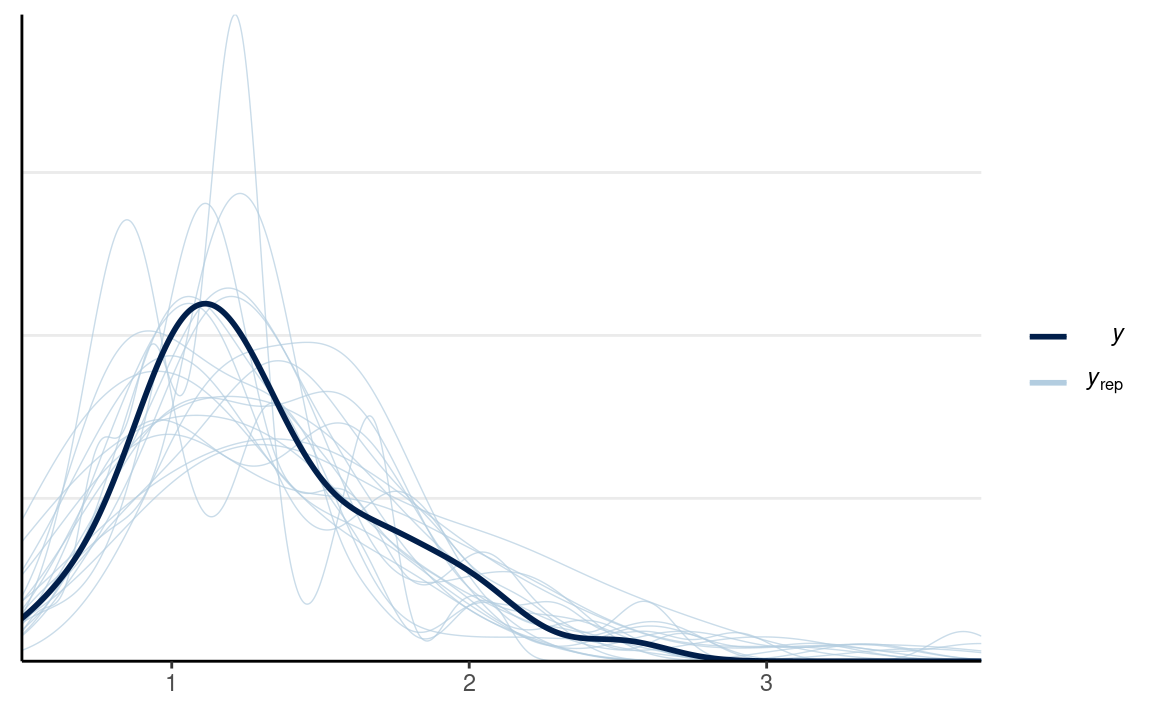
#> convergence, Rhat=1).Notice that \(\nu\) is estimated to be close to 1.
# PPC for Group 2 (vrouw)
y2_tilde <- extract(m0r, pars = "y2_rep")$y2_rep
# Randomly sample 100 data sets (to make plotting faster)
set.seed(2154)
selected_rows <- sample.int(nrow(y2_tilde), size = 100)
ppc_dens_overlay(out_dat$y2,
                 yrep = y2_tilde[selected_rows, ],
                 bw = "SJ")
Bayesian Lognormal Model
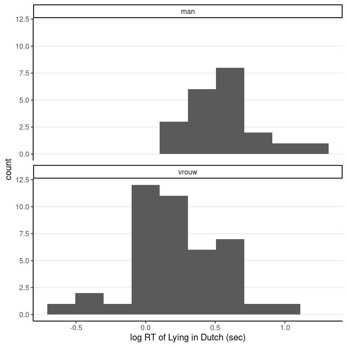
It is not necessary to use a normal model for group comparisons. Indeed, for many problems, the normal model may not be the best option. There has been rich literature on how to model response data. One key issue to address is that response time is non-negative, but a normal model implies that a negative value is always possible. A better option is to assume the logarithm of response time is normally distributed. This implies that the outcome follows a lognormal distribution, which ensures that the outcome will be non-negative. Below is the log-transformed data:
ggplot(lies_cc, aes(x = log(LDMRT_sec))) +
    geom_histogram(bins = 10) +
    facet_wrap(~ Gender,  ncol = 1) +
    labs(x = "log RT of Lying in Dutch (sec)")
Below is a lognormal model with some weak priors:
\[ \begin{aligned} \text{RT}_{i, \text{male}} & \sim \mathrm{Lognormal}(\mu_1, \sigma_1) \\ \text{RT}_{i, \text{female}} & \sim \mathrm{Lognormal}(\mu_2, \sigma_2) \\ \mu_1 & \sim N(0, 1) \\ \mu_2 & \sim N(0, 1) \\ \sigma_1 & \sim N^+(0, 1) \\ \sigma_2 & \sim N^+(0, 1) \end{aligned} \]
data {
  int<lower=0> N1;  // number of observations (group 1)
  int<lower=0> N2;  // number of observations (group 2)
  vector<lower=0>[N1] y1;  // response time (group 1);
  vector<lower=0>[N2] y2;  // response time (group 2);
}
parameters {
  real mu1;  // mean of log(RT) (group 1)
  real<lower=0> sigma1;  // SD of log(RT) (group 1)
  real mu2;  // mean of log(RT) (group 2)
  real<lower=0> sigma2;  // SD of log(RT) (group 2)
}
model {
  // model
  y1 ~ lognormal(mu1, sigma1);
  y2 ~ lognormal(mu2, sigma2);
  // prior
  mu1 ~ normal(0, 1);
  mu2 ~ normal(0, 1);
  sigma1 ~ normal(0, 0.5);
  sigma2 ~ normal(0, 0.5);
}
generated quantities {
  vector<lower=0>[N1] y1_rep;  // place holder
  vector<lower=0>[N2] y2_rep;  // place holder
  for (n in 1:N1)
    y1_rep[n] = lognormal_rng(mu1, sigma1);
  for (n in 1:N2)
    y2_rep[n] = lognormal_rng(mu2, sigma2);
}
Prior Predictive
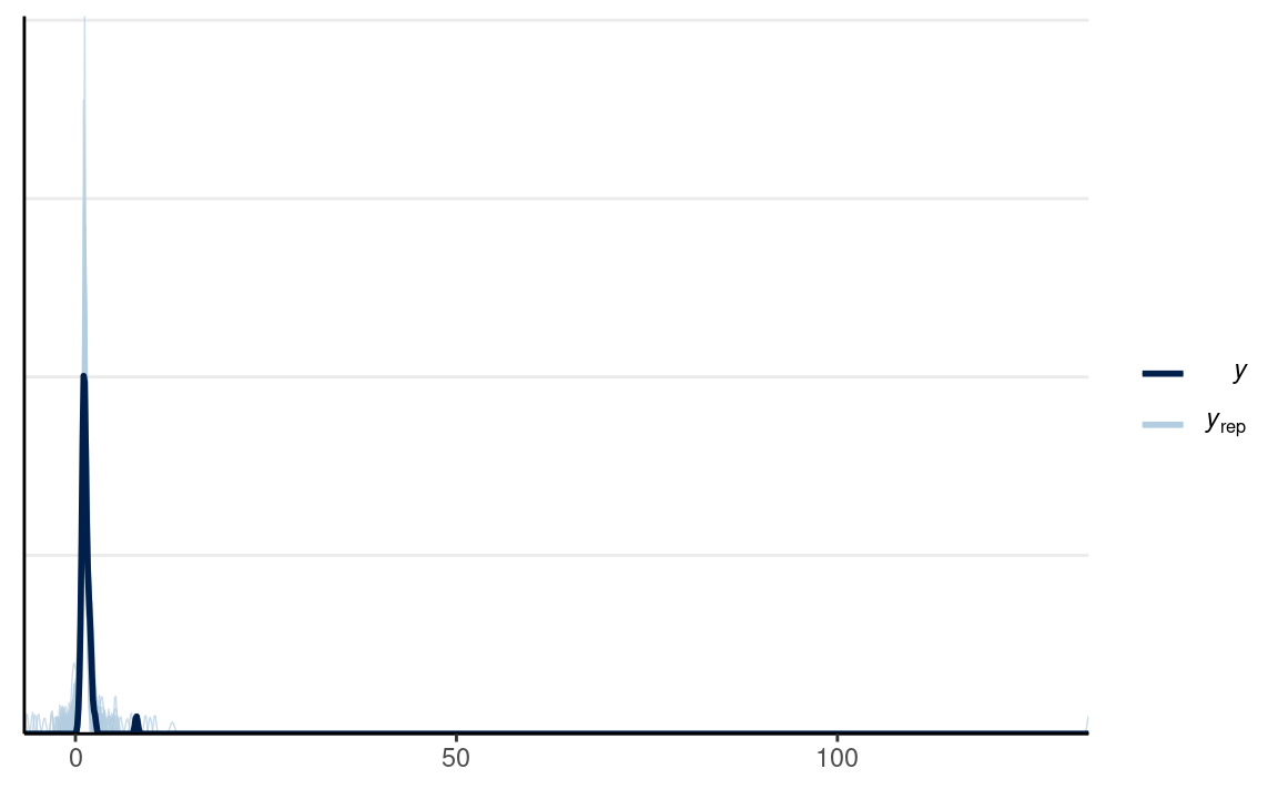
The first time I used \(\mu \sim N(0, 1)\) and \(\sigma \sim N^+(0, 1)\) for both groups.
# Here I use Stan to sample the prior
# 1. form the data list for Stan
m1_dat <- with(lies_cc,
    list(N1 = sum(Gender == "man"),
         N2 = sum(Gender == "vrouw"),
         y1 = LDMRT_sec[which(Gender == "man")],
         y2 = LDMRT_sec[which(Gender == "vrouw")])
)
# 2. Run Stan (with lines for the likelihood commented out)
m1_prior <- stan(
    file = here("stan", "lognormal_2group_prior_only0.stan"),
    data = m1_dat,
    seed = 2151  # for reproducibility
)
#>
#> SAMPLING FOR MODEL 'lognormal_2group_prior_only0' NOW (CHAIN 1).
#> Chain 1:
#> Chain 1: Gradient evaluation took 8e-06 seconds
#> Chain 1: 1000 transitions using 10 leapfrog steps per transition would take 0.08 seconds.
#> Chain 1: Adjust your expectations accordingly!
#> Chain 1:
#> Chain 1:
#> Chain 1: Iteration:    1 / 2000 [  0%]  (Warmup)
#> Chain 1: Iteration:  200 / 2000 [ 10%]  (Warmup)
#> Chain 1: Iteration:  400 / 2000 [ 20%]  (Warmup)
#> Chain 1: Iteration:  600 / 2000 [ 30%]  (Warmup)
#> Chain 1: Iteration:  800 / 2000 [ 40%]  (Warmup)
#> Chain 1: Iteration: 1000 / 2000 [ 50%]  (Warmup)
#> Chain 1: Iteration: 1001 / 2000 [ 50%]  (Sampling)
#> Chain 1: Iteration: 1200 / 2000 [ 60%]  (Sampling)
#> Chain 1: Iteration: 1400 / 2000 [ 70%]  (Sampling)
#> Chain 1: Iteration: 1600 / 2000 [ 80%]  (Sampling)
#> Chain 1: Iteration: 1800 / 2000 [ 90%]  (Sampling)
#> Chain 1: Iteration: 2000 / 2000 [100%]  (Sampling)
#> Chain 1:
#> Chain 1:  Elapsed Time: 0.060325 seconds (Warm-up)
#> Chain 1:                0.034856 seconds (Sampling)
#> Chain 1:                0.095181 seconds (Total)
#> Chain 1:
#>
#> SAMPLING FOR MODEL 'lognormal_2group_prior_only0' NOW (CHAIN 2).
#> Chain 2:
#> Chain 2: Gradient evaluation took 8e-06 seconds
#> Chain 2: 1000 transitions using 10 leapfrog steps per transition would take 0.08 seconds.
#> Chain 2: Adjust your expectations accordingly!
#> Chain 2:
#> Chain 2:
#> Chain 2: Iteration:    1 / 2000 [  0%]  (Warmup)
#> Chain 2: Iteration:  200 / 2000 [ 10%]  (Warmup)
#> Chain 2: Iteration:  400 / 2000 [ 20%]  (Warmup)
#> Chain 2: Iteration:  600 / 2000 [ 30%]  (Warmup)
#> Chain 2: Iteration:  800 / 2000 [ 40%]  (Warmup)
#> Chain 2: Iteration: 1000 / 2000 [ 50%]  (Warmup)
#> Chain 2: Iteration: 1001 / 2000 [ 50%]  (Sampling)
#> Chain 2: Iteration: 1200 / 2000 [ 60%]  (Sampling)
#> Chain 2: Iteration: 1400 / 2000 [ 70%]  (Sampling)
#> Chain 2: Iteration: 1600 / 2000 [ 80%]  (Sampling)
#> Chain 2: Iteration: 1800 / 2000 [ 90%]  (Sampling)
#> Chain 2: Iteration: 2000 / 2000 [100%]  (Sampling)
#> Chain 2:
#> Chain 2:  Elapsed Time: 0.035224 seconds (Warm-up)
#> Chain 2:                0.03869 seconds (Sampling)
#> Chain 2:                0.073914 seconds (Total)
#> Chain 2:
#>
#> SAMPLING FOR MODEL 'lognormal_2group_prior_only0' NOW (CHAIN 3).
#> Chain 3:
#> Chain 3: Gradient evaluation took 1.6e-05 seconds
#> Chain 3: 1000 transitions using 10 leapfrog steps per transition would take 0.16 seconds.
#> Chain 3: Adjust your expectations accordingly!
#> Chain 3:
#> Chain 3:
#> Chain 3: Iteration:    1 / 2000 [  0%]  (Warmup)
#> Chain 3: Iteration:  200 / 2000 [ 10%]  (Warmup)
#> Chain 3: Iteration:  400 / 2000 [ 20%]  (Warmup)
#> Chain 3: Iteration:  600 / 2000 [ 30%]  (Warmup)
#> Chain 3: Iteration:  800 / 2000 [ 40%]  (Warmup)
#> Chain 3: Iteration: 1000 / 2000 [ 50%]  (Warmup)
#> Chain 3: Iteration: 1001 / 2000 [ 50%]  (Sampling)
#> Chain 3: Iteration: 1200 / 2000 [ 60%]  (Sampling)
#> Chain 3: Iteration: 1400 / 2000 [ 70%]  (Sampling)
#> Chain 3: Iteration: 1600 / 2000 [ 80%]  (Sampling)
#> Chain 3: Iteration: 1800 / 2000 [ 90%]  (Sampling)
#> Chain 3: Iteration: 2000 / 2000 [100%]  (Sampling)
#> Chain 3:
#> Chain 3:  Elapsed Time: 0.037544 seconds (Warm-up)
#> Chain 3:                0.034993 seconds (Sampling)
#> Chain 3:                0.072537 seconds (Total)
#> Chain 3:
#>
#> SAMPLING FOR MODEL 'lognormal_2group_prior_only0' NOW (CHAIN 4).
#> Chain 4:
#> Chain 4: Gradient evaluation took 1e-05 seconds
#> Chain 4: 1000 transitions using 10 leapfrog steps per transition would take 0.1 seconds.
#> Chain 4: Adjust your expectations accordingly!
#> Chain 4:
#> Chain 4:
#> Chain 4: Iteration:    1 / 2000 [  0%]  (Warmup)
#> Chain 4: Iteration:  200 / 2000 [ 10%]  (Warmup)
#> Chain 4: Iteration:  400 / 2000 [ 20%]  (Warmup)
#> Chain 4: Iteration:  600 / 2000 [ 30%]  (Warmup)
#> Chain 4: Iteration:  800 / 2000 [ 40%]  (Warmup)
#> Chain 4: Iteration: 1000 / 2000 [ 50%]  (Warmup)
#> Chain 4: Iteration: 1001 / 2000 [ 50%]  (Sampling)
#> Chain 4: Iteration: 1200 / 2000 [ 60%]  (Sampling)
#> Chain 4: Iteration: 1400 / 2000 [ 70%]  (Sampling)
#> Chain 4: Iteration: 1600 / 2000 [ 80%]  (Sampling)
#> Chain 4: Iteration: 1800 / 2000 [ 90%]  (Sampling)
#> Chain 4: Iteration: 2000 / 2000 [100%]  (Sampling)
#> Chain 4:
#> Chain 4:  Elapsed Time: 0.039547 seconds (Warm-up)
#> Chain 4:                0.032211 seconds (Sampling)
#> Chain 4:                0.071758 seconds (Total)
#> Chain 4:
# PPC for Group 1 (man)
y1_tilde <- extract(m1_prior, pars = "y1_rep")$y1_rep
# Randomly sample 100 data sets (to make plotting faster)
set.seed(2154)
selected_rows <- sample.int(nrow(y1_tilde), size = 100)
ppc_dens_overlay(m1_dat$y1,
yrep = y1_tilde[selected_rows, ],
bw = "SJ")
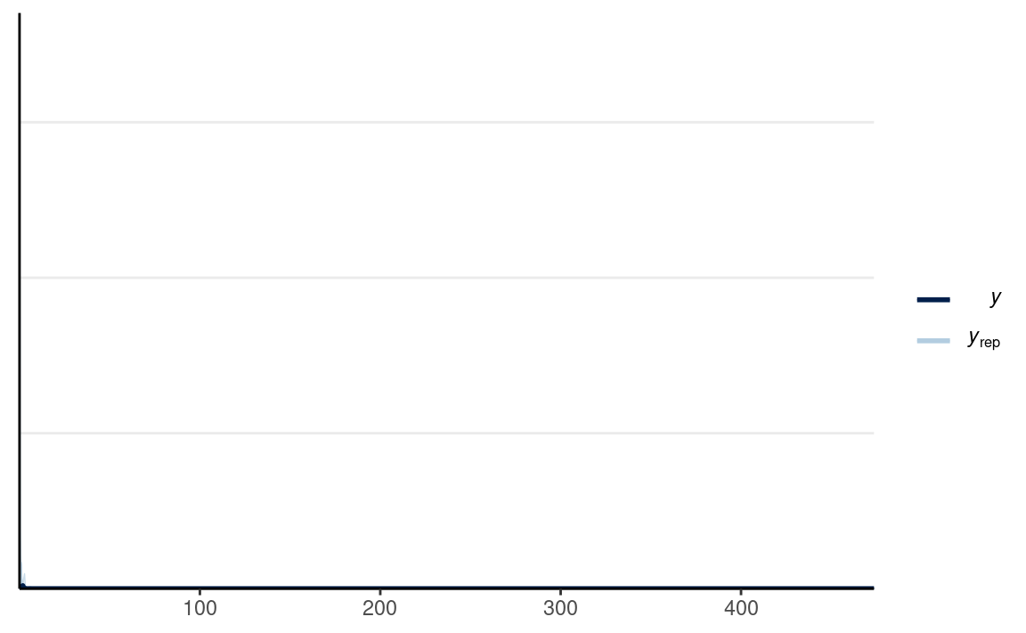
The plot looks off because the priors imply the possibility of very extreme data. I can instead place stronger priors on \(\sigma\) with \(N^+(0, 0.5)\);
m1_prior <- stan(
    file = here("stan", "lognormal_2group_prior_only.stan"),
    data = m1_dat,
    seed = 2151  # for reproducibility
)
#>
#> SAMPLING FOR MODEL 'lognormal_2group_prior_only' NOW (CHAIN 1).
#> Chain 1:
#> Chain 1: Gradient evaluation took 8e-06 seconds
#> Chain 1: 1000 transitions using 10 leapfrog steps per transition would take 0.08 seconds.
#> Chain 1: Adjust your expectations accordingly!
#> Chain 1:
#> Chain 1:
#> Chain 1: Iteration:    1 / 2000 [  0%]  (Warmup)
#> Chain 1: Iteration:  200 / 2000 [ 10%]  (Warmup)
#> Chain 1: Iteration:  400 / 2000 [ 20%]  (Warmup)
#> Chain 1: Iteration:  600 / 2000 [ 30%]  (Warmup)
#> Chain 1: Iteration:  800 / 2000 [ 40%]  (Warmup)
#> Chain 1: Iteration: 1000 / 2000 [ 50%]  (Warmup)
#> Chain 1: Iteration: 1001 / 2000 [ 50%]  (Sampling)
#> Chain 1: Iteration: 1200 / 2000 [ 60%]  (Sampling)
#> Chain 1: Iteration: 1400 / 2000 [ 70%]  (Sampling)
#> Chain 1: Iteration: 1600 / 2000 [ 80%]  (Sampling)
#> Chain 1: Iteration: 1800 / 2000 [ 90%]  (Sampling)
#> Chain 1: Iteration: 2000 / 2000 [100%]  (Sampling)
#> Chain 1:
#> Chain 1:  Elapsed Time: 0.035149 seconds (Warm-up)
#> Chain 1:                0.030669 seconds (Sampling)
#> Chain 1:                0.065818 seconds (Total)
#> Chain 1:
#>
#> SAMPLING FOR MODEL 'lognormal_2group_prior_only' NOW (CHAIN 2).
#> Chain 2:
#> Chain 2: Gradient evaluation took 6e-06 seconds
#> Chain 2: 1000 transitions using 10 leapfrog steps per transition would take 0.06 seconds.
#> Chain 2: Adjust your expectations accordingly!
#> Chain 2:
#> Chain 2:
#> Chain 2: Iteration:    1 / 2000 [  0%]  (Warmup)
#> Chain 2: Iteration:  200 / 2000 [ 10%]  (Warmup)
#> Chain 2: Iteration:  400 / 2000 [ 20%]  (Warmup)
#> Chain 2: Iteration:  600 / 2000 [ 30%]  (Warmup)
#> Chain 2: Iteration:  800 / 2000 [ 40%]  (Warmup)
#> Chain 2: Iteration: 1000 / 2000 [ 50%]  (Warmup)
#> Chain 2: Iteration: 1001 / 2000 [ 50%]  (Sampling)
#> Chain 2: Iteration: 1200 / 2000 [ 60%]  (Sampling)
#> Chain 2: Iteration: 1400 / 2000 [ 70%]  (Sampling)
#> Chain 2: Iteration: 1600 / 2000 [ 80%]  (Sampling)
#> Chain 2: Iteration: 1800 / 2000 [ 90%]  (Sampling)
#> Chain 2: Iteration: 2000 / 2000 [100%]  (Sampling)
#> Chain 2:
#> Chain 2:  Elapsed Time: 0.034002 seconds (Warm-up)
#> Chain 2:                0.03404 seconds (Sampling)
#> Chain 2:                0.068042 seconds (Total)
#> Chain 2:
#>
#> SAMPLING FOR MODEL 'lognormal_2group_prior_only' NOW (CHAIN 3).
#> Chain 3:
#> Chain 3: Gradient evaluation took 8e-06 seconds
#> Chain 3: 1000 transitions using 10 leapfrog steps per transition would take 0.08 seconds.
#> Chain 3: Adjust your expectations accordingly!
#> Chain 3:
#> Chain 3:
#> Chain 3: Iteration:    1 / 2000 [  0%]  (Warmup)
#> Chain 3: Iteration:  200 / 2000 [ 10%]  (Warmup)
#> Chain 3: Iteration:  400 / 2000 [ 20%]  (Warmup)
#> Chain 3: Iteration:  600 / 2000 [ 30%]  (Warmup)
#> Chain 3: Iteration:  800 / 2000 [ 40%]  (Warmup)
#> Chain 3: Iteration: 1000 / 2000 [ 50%]  (Warmup)
#> Chain 3: Iteration: 1001 / 2000 [ 50%]  (Sampling)
#> Chain 3: Iteration: 1200 / 2000 [ 60%]  (Sampling)
#> Chain 3: Iteration: 1400 / 2000 [ 70%]  (Sampling)
#> Chain 3: Iteration: 1600 / 2000 [ 80%]  (Sampling)
#> Chain 3: Iteration: 1800 / 2000 [ 90%]  (Sampling)
#> Chain 3: Iteration: 2000 / 2000 [100%]  (Sampling)
#> Chain 3:
#> Chain 3:  Elapsed Time: 0.034935 seconds (Warm-up)
#> Chain 3:                0.028403 seconds (Sampling)
#> Chain 3:                0.063338 seconds (Total)
#> Chain 3:
#>
#> SAMPLING FOR MODEL 'lognormal_2group_prior_only' NOW (CHAIN 4).
#> Chain 4:
#> Chain 4: Gradient evaluation took 6e-06 seconds
#> Chain 4: 1000 transitions using 10 leapfrog steps per transition would take 0.06 seconds.
#> Chain 4: Adjust your expectations accordingly!
#> Chain 4:
#> Chain 4:
#> Chain 4: Iteration:    1 / 2000 [  0%]  (Warmup)
#> Chain 4: Iteration:  200 / 2000 [ 10%]  (Warmup)
#> Chain 4: Iteration:  400 / 2000 [ 20%]  (Warmup)
#> Chain 4: Iteration:  600 / 2000 [ 30%]  (Warmup)
#> Chain 4: Iteration:  800 / 2000 [ 40%]  (Warmup)
#> Chain 4: Iteration: 1000 / 2000 [ 50%]  (Warmup)
#> Chain 4: Iteration: 1001 / 2000 [ 50%]  (Sampling)
#> Chain 4: Iteration: 1200 / 2000 [ 60%]  (Sampling)
#> Chain 4: Iteration: 1400 / 2000 [ 70%]  (Sampling)
#> Chain 4: Iteration: 1600 / 2000 [ 80%]  (Sampling)
#> Chain 4: Iteration: 1800 / 2000 [ 90%]  (Sampling)
#> Chain 4: Iteration: 2000 / 2000 [100%]  (Sampling)
#> Chain 4:
#> Chain 4:  Elapsed Time: 0.029862 seconds (Warm-up)
#> Chain 4:                0.029072 seconds (Sampling)
#> Chain 4:                0.058934 seconds (Total)
#> Chain 4:
# PPC for Group 1 (man) and Group 2 (vrouw)
y1_tilde <- extract(m1_prior, pars = "y1_rep")$y1_rep
y2_tilde <- extract(m1_prior, pars = "y2_rep")$y2_rep
# Randomly sample 100 data sets (to make plotting faster)
set.seed(2154)
selected_rows <- sample.int(nrow(y1_tilde), size = 100)
ppc_dens_overlay(m1_dat$y1,
yrep = y1_tilde[selected_rows, ],
bw = "SJ")
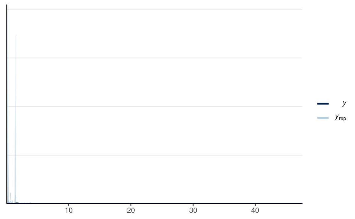
ppc_dens_overlay(m1_dat$y2,
                 yrep = y2_tilde[selected_rows, ],
                 bw = "SJ")
which looks a bit better in terms of capturing what is possible, although one can argue it still wouldn’t make sense to have observations with RT more than 10 seconds.
MCMC Sampling
Let’s feed the data to rstan.
m1 <- stan(here("stan", "lognormal_2group.stan"),
    data = m1_dat,
    seed = 2151,  # for reproducibility
    iter = 4000
)
#>
#> SAMPLING FOR MODEL 'lognormal_2group' NOW (CHAIN 1).
#> Chain 1:
#> Chain 1: Gradient evaluation took 1.1e-05 seconds
#> Chain 1: 1000 transitions using 10 leapfrog steps per transition would take 0.11 seconds.
#> Chain 1: Adjust your expectations accordingly!
#> Chain 1:
#> Chain 1:
#> Chain 1: Iteration:    1 / 4000 [  0%]  (Warmup)
#> Chain 1: Iteration:  400 / 4000 [ 10%]  (Warmup)
#> Chain 1: Iteration:  800 / 4000 [ 20%]  (Warmup)
#> Chain 1: Iteration: 1200 / 4000 [ 30%]  (Warmup)
#> Chain 1: Iteration: 1600 / 4000 [ 40%]  (Warmup)
#> Chain 1: Iteration: 2000 / 4000 [ 50%]  (Warmup)
#> Chain 1: Iteration: 2001 / 4000 [ 50%]  (Sampling)
#> Chain 1: Iteration: 2400 / 4000 [ 60%]  (Sampling)
#> Chain 1: Iteration: 2800 / 4000 [ 70%]  (Sampling)
#> Chain 1: Iteration: 3200 / 4000 [ 80%]  (Sampling)
#> Chain 1: Iteration: 3600 / 4000 [ 90%]  (Sampling)
#> Chain 1: Iteration: 4000 / 4000 [100%]  (Sampling)
#> Chain 1:
#> Chain 1:  Elapsed Time: 0.063718 seconds (Warm-up)
#> Chain 1:                0.069889 seconds (Sampling)
#> Chain 1:                0.133607 seconds (Total)
#> Chain 1:
#>
#> SAMPLING FOR MODEL 'lognormal_2group' NOW (CHAIN 2).
#> Chain 2:
#> Chain 2: Gradient evaluation took 1e-05 seconds
#> Chain 2: 1000 transitions using 10 leapfrog steps per transition would take 0.1 seconds.
#> Chain 2: Adjust your expectations accordingly!
#> Chain 2:
#> Chain 2:
#> Chain 2: Iteration:    1 / 4000 [  0%]  (Warmup)
#> Chain 2: Iteration:  400 / 4000 [ 10%]  (Warmup)
#> Chain 2: Iteration:  800 / 4000 [ 20%]  (Warmup)
#> Chain 2: Iteration: 1200 / 4000 [ 30%]  (Warmup)
#> Chain 2: Iteration: 1600 / 4000 [ 40%]  (Warmup)
#> Chain 2: Iteration: 2000 / 4000 [ 50%]  (Warmup)
#> Chain 2: Iteration: 2001 / 4000 [ 50%]  (Sampling)
#> Chain 2: Iteration: 2400 / 4000 [ 60%]  (Sampling)
#> Chain 2: Iteration: 2800 / 4000 [ 70%]  (Sampling)
#> Chain 2: Iteration: 3200 / 4000 [ 80%]  (Sampling)
#> Chain 2: Iteration: 3600 / 4000 [ 90%]  (Sampling)
#> Chain 2: Iteration: 4000 / 4000 [100%]  (Sampling)
#> Chain 2:
#> Chain 2:  Elapsed Time: 0.066228 seconds (Warm-up)
#> Chain 2:                0.0747 seconds (Sampling)
#> Chain 2:                0.140928 seconds (Total)
#> Chain 2:
#>
#> SAMPLING FOR MODEL 'lognormal_2group' NOW (CHAIN 3).
#> Chain 3:
#> Chain 3: Gradient evaluation took 1.2e-05 seconds
#> Chain 3: 1000 transitions using 10 leapfrog steps per transition would take 0.12 seconds.
#> Chain 3: Adjust your expectations accordingly!
#> Chain 3:
#> Chain 3:
#> Chain 3: Iteration:    1 / 4000 [  0%]  (Warmup)
#> Chain 3: Iteration:  400 / 4000 [ 10%]  (Warmup)
#> Chain 3: Iteration:  800 / 4000 [ 20%]  (Warmup)
#> Chain 3: Iteration: 1200 / 4000 [ 30%]  (Warmup)
#> Chain 3: Iteration: 1600 / 4000 [ 40%]  (Warmup)
#> Chain 3: Iteration: 2000 / 4000 [ 50%]  (Warmup)
#> Chain 3: Iteration: 2001 / 4000 [ 50%]  (Sampling)
#> Chain 3: Iteration: 2400 / 4000 [ 60%]  (Sampling)
#> Chain 3: Iteration: 2800 / 4000 [ 70%]  (Sampling)
#> Chain 3: Iteration: 3200 / 4000 [ 80%]  (Sampling)
#> Chain 3: Iteration: 3600 / 4000 [ 90%]  (Sampling)
#> Chain 3: Iteration: 4000 / 4000 [100%]  (Sampling)
#> Chain 3:
#> Chain 3:  Elapsed Time: 0.063543 seconds (Warm-up)
#> Chain 3:                0.069512 seconds (Sampling)
#> Chain 3:                0.133055 seconds (Total)
#> Chain 3:
#>
#> SAMPLING FOR MODEL 'lognormal_2group' NOW (CHAIN 4).
#> Chain 4:
#> Chain 4: Gradient evaluation took 8e-06 seconds
#> Chain 4: 1000 transitions using 10 leapfrog steps per transition would take 0.08 seconds.
#> Chain 4: Adjust your expectations accordingly!
#> Chain 4:
#> Chain 4:
#> Chain 4: Iteration:    1 / 4000 [  0%]  (Warmup)
#> Chain 4: Iteration:  400 / 4000 [ 10%]  (Warmup)
#> Chain 4: Iteration:  800 / 4000 [ 20%]  (Warmup)
#> Chain 4: Iteration: 1200 / 4000 [ 30%]  (Warmup)
#> Chain 4: Iteration: 1600 / 4000 [ 40%]  (Warmup)
#> Chain 4: Iteration: 2000 / 4000 [ 50%]  (Warmup)
#> Chain 4: Iteration: 2001 / 4000 [ 50%]  (Sampling)
#> Chain 4: Iteration: 2400 / 4000 [ 60%]  (Sampling)
#> Chain 4: Iteration: 2800 / 4000 [ 70%]  (Sampling)
#> Chain 4: Iteration: 3200 / 4000 [ 80%]  (Sampling)
#> Chain 4: Iteration: 3600 / 4000 [ 90%]  (Sampling)
#> Chain 4: Iteration: 4000 / 4000 [100%]  (Sampling)
#> Chain 4:
#> Chain 4:  Elapsed Time: 0.074646 seconds (Warm-up)
#> Chain 4:                0.074334 seconds (Sampling)
#> Chain 4:                0.14898 seconds (Total)
#> Chain 4:
We can summarize the posterior:
m1_summary <- as.array(m1,
                       pars = c("mu1", "sigma1", "mu2", "sigma2")) %>%
    summarize_draws()
It appears that \(\mu\) is much larger for man than for women. You can obtain the posterior for \(\mu_2 - \mu_1\) to check:
as.array(m1, pars = c("mu1", "sigma1", "mu2", "sigma2")) %>%
    as_draws() %>%
    mutate_variables(dmu = mu2 - mu1) %>%
    summarize_draws()
#> # A tibble: 5 × 10
#>   variable   mean median     sd    mad     q5    q95  rhat ess_bulk
#>   <chr>     <dbl>  <dbl>  <dbl>  <dbl>  <dbl>  <dbl> <dbl>    <dbl>
#> 1 mu1       0.560  0.560 0.0614 0.0594  0.462  0.661  1.00    7581.
#> 2 sigma1    0.270  0.263 0.0474 0.0432  0.207  0.356  1.00    7121.
#> 3 mu2       0.207  0.208 0.0516 0.0504  0.122  0.292  1.00    7781.
#> 4 sigma2    0.334  0.331 0.0376 0.0360  0.278  0.400  1.00    8605.
#> 5 dmu      -0.353 -0.353 0.0798 0.0774 -0.485 -0.223  1.00    7465.
#> # … with 1 more variable: ess_tail <dbl>
We can show some visual as well:
From the normal model, it was estimated that the mean log(RT) for lying in Dutch was 0.56 log(seconds), 90% CI [0.46, 0.66]. On average, women had faster log(RT) when asked to tell lies in Dutch than mens, with the mean log(RT) for women being 0.27 log(seconds), 90% CI [0.21, 0.36].
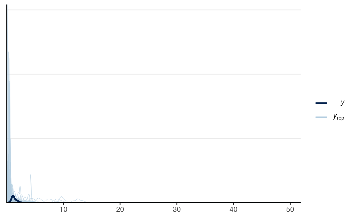
Posterior Predictive Check
Densities
We can first check the densities:
y1_tilde <- rstan::extract(m1, pars = "y1_rep")$y1_rep
y2_tilde <- rstan::extract(m1, pars = "y2_rep")$y2_rep
# Randomly sample 20 data sets (for faster plotting)
selected_rows <- sample.int(nrow(y1_tilde), size = 20)
ppc_dens_overlay(m1_dat$y1,
                 yrep = y1_tilde[selected_rows, ],
                 bw = "SJ")
ppc_dens_overlay(m1_dat$y2,
                 yrep = y2_tilde[selected_rows, ],
                 bw = "SJ")
Minimum
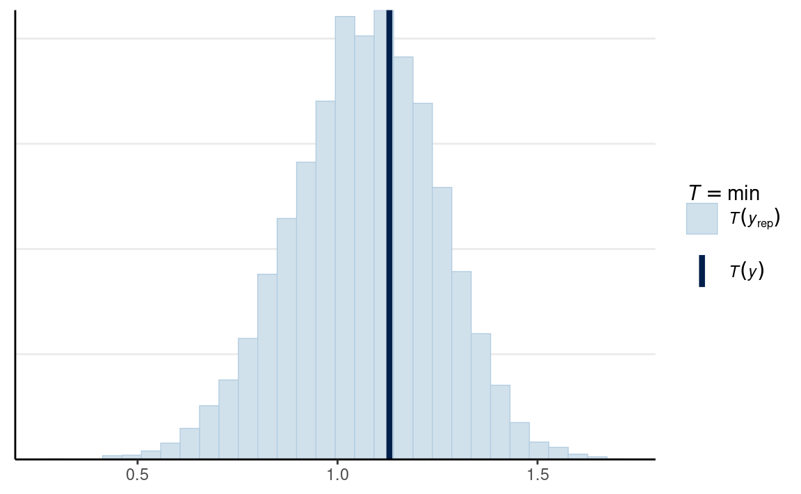
For response time data, one thing that would be important is the minimum of the data, as the lognormal model implies that it is possible to have an RT close to zero. In a lot of tasks, on the other end, the minimum is much larger than the 0 because there is a limit on how fast a person can respond to a task.
# Man
ppc_stat(
  m1_dat$y1,
  yrep = y1_tilde,
  stat = min
)
# Vrouw
ppc_stat(
  m1_dat$y2,
  yrep = y2_tilde,
  stat = min
)
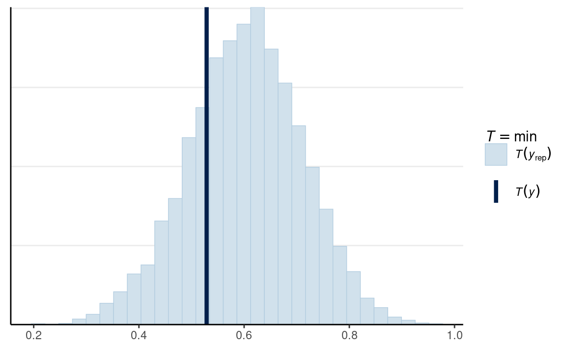
In this case, the minimum of the data was within the range of what the model would predict.
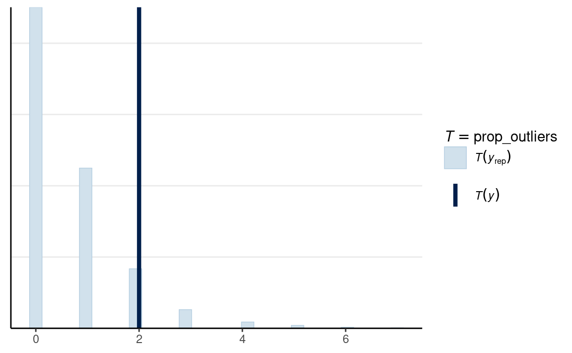
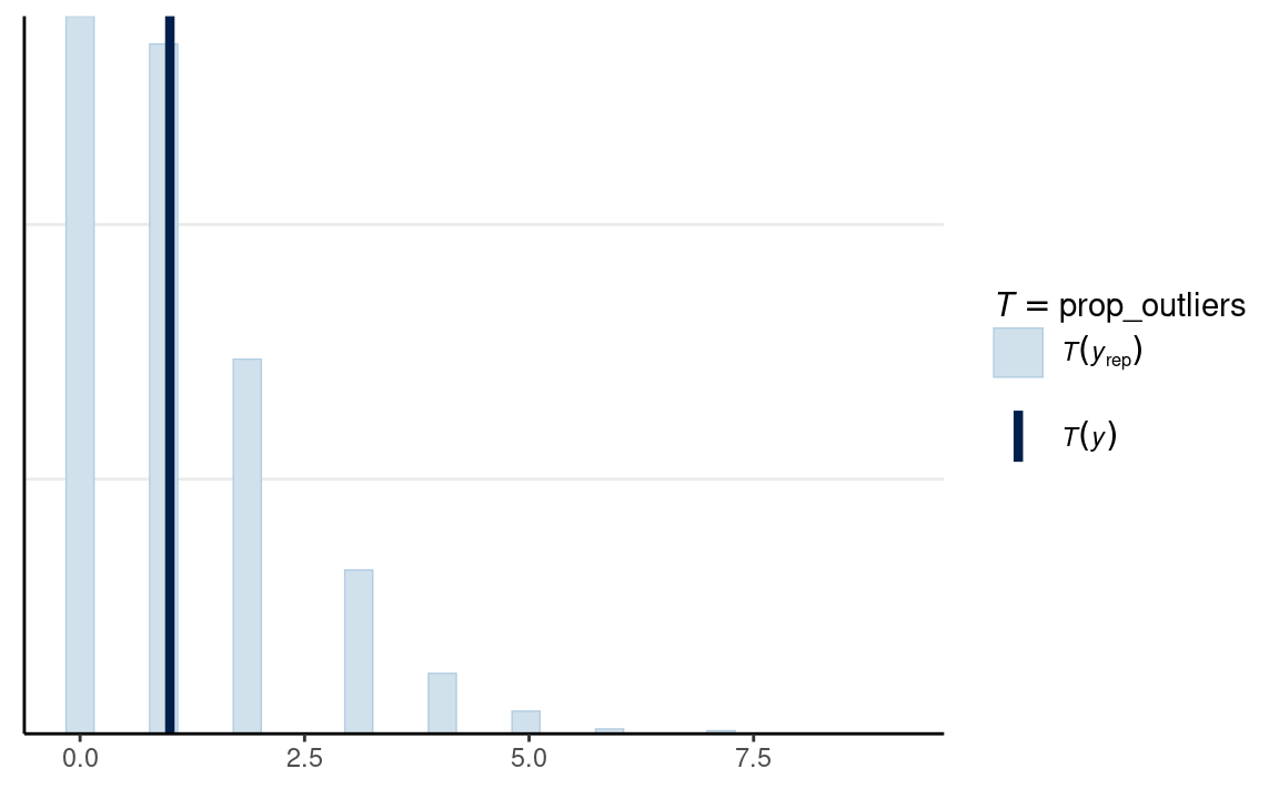
Proportion Outliers
Another check we can perform is in predicting the proportion of outliers.
# Function for number of outliers
prop_outliers <- function(x) {
  length(boxplot.stats(x)$out)
}
# Man
ppc_stat(
  m1_dat$y1,
  yrep = y1_tilde,
  stat = prop_outliers
)
# Vrouw
ppc_stat(
  m1_dat$y2,
  yrep = y2_tilde,
  stat = prop_outliers
)
Use Difference As Parameter
The above model has \(\mu_1\) and \(\mu_2\) as parameters, and \(\delta = \mu_2 - \mu_1\) as a derived quantify from the parameters. We can instead treat \(\mu_1\) and \(\delta\) as parameters, and \(\mu_2 = \mu_1 + \delta\) as a derived quantity. We can also impose the homogeneity of variance assumption, as shown below, although it is usually not advisable in a two-group setting:
\[ \begin{aligned} \text{RT}_{i, \text{male}} & \sim \mathrm{Lognormal}(\mu_1, \sigma) \\ \text{RT}_{i, \text{female}} & \sim \mathrm{Lognormal}(\mu_1 + \delta, \sigma) \\ \mu_1 & \sim N(0, 1) \\ \delta & \sim N(0, 1) \\ \sigma & \sim N^+(0, 0.5) \end{aligned} \]
m2 <- stan(here("stan", "lognormal_diff.stan"),
    data = m1_dat,
    seed = 1922,  # for reproducibility
    iter = 4000
)
#>
#> SAMPLING FOR MODEL 'lognormal_diff' NOW (CHAIN 1).
#> Chain 1:
#> Chain 1: Gradient evaluation took 9e-06 seconds
#> Chain 1: 1000 transitions using 10 leapfrog steps per transition would take 0.09 seconds.
#> Chain 1: Adjust your expectations accordingly!
#> Chain 1:
#> Chain 1:
#> Chain 1: Iteration:    1 / 4000 [  0%]  (Warmup)
#> Chain 1: Iteration:  400 / 4000 [ 10%]  (Warmup)
#> Chain 1: Iteration:  800 / 4000 [ 20%]  (Warmup)
#> Chain 1: Iteration: 1200 / 4000 [ 30%]  (Warmup)
#> Chain 1: Iteration: 1600 / 4000 [ 40%]  (Warmup)
#> Chain 1: Iteration: 2000 / 4000 [ 50%]  (Warmup)
#> Chain 1: Iteration: 2001 / 4000 [ 50%]  (Sampling)
#> Chain 1: Iteration: 2400 / 4000 [ 60%]  (Sampling)
#> Chain 1: Iteration: 2800 / 4000 [ 70%]  (Sampling)
#> Chain 1: Iteration: 3200 / 4000 [ 80%]  (Sampling)
#> Chain 1: Iteration: 3600 / 4000 [ 90%]  (Sampling)
#> Chain 1: Iteration: 4000 / 4000 [100%]  (Sampling)
#> Chain 1:
#> Chain 1:  Elapsed Time: 0.075794 seconds (Warm-up)
#> Chain 1:                0.079339 seconds (Sampling)
#> Chain 1:                0.155133 seconds (Total)
#> Chain 1:
#>
#> SAMPLING FOR MODEL 'lognormal_diff' NOW (CHAIN 2).
#> Chain 2:
#> Chain 2: Gradient evaluation took 1.1e-05 seconds
#> Chain 2: 1000 transitions using 10 leapfrog steps per transition would take 0.11 seconds.
#> Chain 2: Adjust your expectations accordingly!
#> Chain 2:
#> Chain 2:
#> Chain 2: Iteration:    1 / 4000 [  0%]  (Warmup)
#> Chain 2: Iteration:  400 / 4000 [ 10%]  (Warmup)
#> Chain 2: Iteration:  800 / 4000 [ 20%]  (Warmup)
#> Chain 2: Iteration: 1200 / 4000 [ 30%]  (Warmup)
#> Chain 2: Iteration: 1600 / 4000 [ 40%]  (Warmup)
#> Chain 2: Iteration: 2000 / 4000 [ 50%]  (Warmup)
#> Chain 2: Iteration: 2001 / 4000 [ 50%]  (Sampling)
#> Chain 2: Iteration: 2400 / 4000 [ 60%]  (Sampling)
#> Chain 2: Iteration: 2800 / 4000 [ 70%]  (Sampling)
#> Chain 2: Iteration: 3200 / 4000 [ 80%]  (Sampling)
#> Chain 2: Iteration: 3600 / 4000 [ 90%]  (Sampling)
#> Chain 2: Iteration: 4000 / 4000 [100%]  (Sampling)
#> Chain 2:
#> Chain 2:  Elapsed Time: 0.082047 seconds (Warm-up)
#> Chain 2:                0.080891 seconds (Sampling)
#> Chain 2:                0.162938 seconds (Total)
#> Chain 2:
#>
#> SAMPLING FOR MODEL 'lognormal_diff' NOW (CHAIN 3).
#> Chain 3:
#> Chain 3: Gradient evaluation took 1e-05 seconds
#> Chain 3: 1000 transitions using 10 leapfrog steps per transition would take 0.1 seconds.
#> Chain 3: Adjust your expectations accordingly!
#> Chain 3:
#> Chain 3:
#> Chain 3: Iteration:    1 / 4000 [  0%]  (Warmup)
#> Chain 3: Iteration:  400 / 4000 [ 10%]  (Warmup)
#> Chain 3: Iteration:  800 / 4000 [ 20%]  (Warmup)
#> Chain 3: Iteration: 1200 / 4000 [ 30%]  (Warmup)
#> Chain 3: Iteration: 1600 / 4000 [ 40%]  (Warmup)
#> Chain 3: Iteration: 2000 / 4000 [ 50%]  (Warmup)
#> Chain 3: Iteration: 2001 / 4000 [ 50%]  (Sampling)
#> Chain 3: Iteration: 2400 / 4000 [ 60%]  (Sampling)
#> Chain 3: Iteration: 2800 / 4000 [ 70%]  (Sampling)
#> Chain 3: Iteration: 3200 / 4000 [ 80%]  (Sampling)
#> Chain 3: Iteration: 3600 / 4000 [ 90%]  (Sampling)
#> Chain 3: Iteration: 4000 / 4000 [100%]  (Sampling)
#> Chain 3:
#> Chain 3:  Elapsed Time: 0.078592 seconds (Warm-up)
#> Chain 3:                0.090809 seconds (Sampling)
#> Chain 3:                0.169401 seconds (Total)
#> Chain 3:
#>
#> SAMPLING FOR MODEL 'lognormal_diff' NOW (CHAIN 4).
#> Chain 4:
#> Chain 4: Gradient evaluation took 9e-06 seconds
#> Chain 4: 1000 transitions using 10 leapfrog steps per transition would take 0.09 seconds.
#> Chain 4: Adjust your expectations accordingly!
#> Chain 4:
#> Chain 4:
#> Chain 4: Iteration:    1 / 4000 [  0%]  (Warmup)
#> Chain 4: Iteration:  400 / 4000 [ 10%]  (Warmup)
#> Chain 4: Iteration:  800 / 4000 [ 20%]  (Warmup)
#> Chain 4: Iteration: 1200 / 4000 [ 30%]  (Warmup)
#> Chain 4: Iteration: 1600 / 4000 [ 40%]  (Warmup)
#> Chain 4: Iteration: 2000 / 4000 [ 50%]  (Warmup)
#> Chain 4: Iteration: 2001 / 4000 [ 50%]  (Sampling)
#> Chain 4: Iteration: 2400 / 4000 [ 60%]  (Sampling)
#> Chain 4: Iteration: 2800 / 4000 [ 70%]  (Sampling)
#> Chain 4: Iteration: 3200 / 4000 [ 80%]  (Sampling)
#> Chain 4: Iteration: 3600 / 4000 [ 90%]  (Sampling)
#> Chain 4: Iteration: 4000 / 4000 [100%]  (Sampling)
#> Chain 4:
#> Chain 4:  Elapsed Time: 0.083919 seconds (Warm-up)
#> Chain 4:                0.091004 seconds (Sampling)
#> Chain 4:                0.174923 seconds (Total)
#> Chain 4:#> Inference for Stan model: lognormal_diff.
#> 4 chains, each with iter=4000; warmup=2000; thin=1;
#> post-warmup draws per chain=2000, total post-warmup draws=8000.
#>
#> mean se_mean sd 2.5% 25% 50% 75% 97.5% n_eff Rhat
#> mu1 0.56 0 0.07 0.43 0.51 0.56 0.60 0.69 3704 1
#> dmu -0.35 0 0.08 -0.51 -0.40 -0.35 -0.29 -0.19 3635 1
#> sigma 0.31 0 0.03 0.26 0.29 0.31 0.33 0.37 4292 1
#> mu2 0.21 0 0.05 0.12 0.18 0.21 0.24 0.30 8734 1
#>
#> Samples were drawn using NUTS(diag_e) at Thu Apr 28 11:39:44 2022.
#> For each parameter, n_eff is a crude measure of effective sample size,
#> and Rhat is the potential scale reduction factor on split chains (at
#> convergence, Rhat=1).Within-Subject
This is similar to a paired \(t\) test, but uses a lognormal distribution.
\[\begin{align} \text{LDMRT}_{i} & \sim \mathrm{Lognormal}(\theta_i, \sigma) \\ \text{LEMRT}_{i} & \sim \mathrm{Lognormal}(\theta_i + \delta, \sigma) \\ \theta_i & = \mu_1 + \tau \eta_i \\ \eta_i & \sim N(0, 1) \\ \mu_1 & \sim N(0, 1) \\ \delta & \sim N(0, 1) \\ \sigma & \sim N^+(0, 0.5) \\ \tau & \sim t^+(4, 0, 0.5) \end{align}\]
Parameters:
- \(\mu_1\): mean parameter for log(RT) for lying in Dutch condition
- \(\delta\): mean difference in log(RT) between the lying in English and lying in Dutch
- \(\sigma\): within-person standard deviation of log(RT)
- \(\eta_1\), \(\ldots\), \(\eta_{63}\): z-scores for individual mean response time
- \(\tau\): standard deviation of individual differences
This is an example of a hierarchical model with a non-centered parameterization (using \(\eta\) instead of \(\theta\) as a parameter). We’re letting the data update our belief on how much individual difference there is.
m3_dat <- with(lies_cc,
    list(N = length(LDMRT_sec),
         y1 = LDMRT_sec,
         y2 = LEMRT_sec)
)
m3 <- stan(here("stan", "within-subjects_lognorm.stan"),
    data = m3_dat,
    seed = 2151,  # for reproducibility
    iter = 4000,
    control = list(adapt_delta = .95)
)
#>
#> SAMPLING FOR MODEL 'within-subjects_lognorm' NOW (CHAIN 1).
#> Chain 1:
#> Chain 1: Gradient evaluation took 2.3e-05 seconds
#> Chain 1: 1000 transitions using 10 leapfrog steps per transition would take 0.23 seconds.
#> Chain 1: Adjust your expectations accordingly!
#> Chain 1:
#> Chain 1:
#> Chain 1: Iteration:    1 / 4000 [  0%]  (Warmup)
#> Chain 1: Iteration:  400 / 4000 [ 10%]  (Warmup)
#> Chain 1: Iteration:  800 / 4000 [ 20%]  (Warmup)
#> Chain 1: Iteration: 1200 / 4000 [ 30%]  (Warmup)
#> Chain 1: Iteration: 1600 / 4000 [ 40%]  (Warmup)
#> Chain 1: Iteration: 2000 / 4000 [ 50%]  (Warmup)
#> Chain 1: Iteration: 2001 / 4000 [ 50%]  (Sampling)
#> Chain 1: Iteration: 2400 / 4000 [ 60%]  (Sampling)
#> Chain 1: Iteration: 2800 / 4000 [ 70%]  (Sampling)
#> Chain 1: Iteration: 3200 / 4000 [ 80%]  (Sampling)
#> Chain 1: Iteration: 3600 / 4000 [ 90%]  (Sampling)
#> Chain 1: Iteration: 4000 / 4000 [100%]  (Sampling)
#> Chain 1:
#> Chain 1:  Elapsed Time: 1.12389 seconds (Warm-up)
#> Chain 1:                0.927768 seconds (Sampling)
#> Chain 1:                2.05166 seconds (Total)
#> Chain 1:
#>
#> SAMPLING FOR MODEL 'within-subjects_lognorm' NOW (CHAIN 2).
#> Chain 2:
#> Chain 2: Gradient evaluation took 2.1e-05 seconds
#> Chain 2: 1000 transitions using 10 leapfrog steps per transition would take 0.21 seconds.
#> Chain 2: Adjust your expectations accordingly!
#> Chain 2:
#> Chain 2:
#> Chain 2: Iteration:    1 / 4000 [  0%]  (Warmup)
#> Chain 2: Iteration:  400 / 4000 [ 10%]  (Warmup)
#> Chain 2: Iteration:  800 / 4000 [ 20%]  (Warmup)
#> Chain 2: Iteration: 1200 / 4000 [ 30%]  (Warmup)
#> Chain 2: Iteration: 1600 / 4000 [ 40%]  (Warmup)
#> Chain 2: Iteration: 2000 / 4000 [ 50%]  (Warmup)
#> Chain 2: Iteration: 2001 / 4000 [ 50%]  (Sampling)
#> Chain 2: Iteration: 2400 / 4000 [ 60%]  (Sampling)
#> Chain 2: Iteration: 2800 / 4000 [ 70%]  (Sampling)
#> Chain 2: Iteration: 3200 / 4000 [ 80%]  (Sampling)
#> Chain 2: Iteration: 3600 / 4000 [ 90%]  (Sampling)
#> Chain 2: Iteration: 4000 / 4000 [100%]  (Sampling)
#> Chain 2:
#> Chain 2:  Elapsed Time: 1.04517 seconds (Warm-up)
#> Chain 2:                0.939345 seconds (Sampling)
#> Chain 2:                1.98452 seconds (Total)
#> Chain 2:
#>
#> SAMPLING FOR MODEL 'within-subjects_lognorm' NOW (CHAIN 3).
#> Chain 3:
#> Chain 3: Gradient evaluation took 2.3e-05 seconds
#> Chain 3: 1000 transitions using 10 leapfrog steps per transition would take 0.23 seconds.
#> Chain 3: Adjust your expectations accordingly!
#> Chain 3:
#> Chain 3:
#> Chain 3: Iteration:    1 / 4000 [  0%]  (Warmup)
#> Chain 3: Iteration:  400 / 4000 [ 10%]  (Warmup)
#> Chain 3: Iteration:  800 / 4000 [ 20%]  (Warmup)
#> Chain 3: Iteration: 1200 / 4000 [ 30%]  (Warmup)
#> Chain 3: Iteration: 1600 / 4000 [ 40%]  (Warmup)
#> Chain 3: Iteration: 2000 / 4000 [ 50%]  (Warmup)
#> Chain 3: Iteration: 2001 / 4000 [ 50%]  (Sampling)
#> Chain 3: Iteration: 2400 / 4000 [ 60%]  (Sampling)
#> Chain 3: Iteration: 2800 / 4000 [ 70%]  (Sampling)
#> Chain 3: Iteration: 3200 / 4000 [ 80%]  (Sampling)
#> Chain 3: Iteration: 3600 / 4000 [ 90%]  (Sampling)
#> Chain 3: Iteration: 4000 / 4000 [100%]  (Sampling)
#> Chain 3:
#> Chain 3:  Elapsed Time: 1.21053 seconds (Warm-up)
#> Chain 3:                0.952319 seconds (Sampling)
#> Chain 3:                2.16285 seconds (Total)
#> Chain 3:
#>
#> SAMPLING FOR MODEL 'within-subjects_lognorm' NOW (CHAIN 4).
#> Chain 4:
#> Chain 4: Gradient evaluation took 2.5e-05 seconds
#> Chain 4: 1000 transitions using 10 leapfrog steps per transition would take 0.25 seconds.
#> Chain 4: Adjust your expectations accordingly!
#> Chain 4:
#> Chain 4:
#> Chain 4: Iteration:    1 / 4000 [  0%]  (Warmup)
#> Chain 4: Iteration:  400 / 4000 [ 10%]  (Warmup)
#> Chain 4: Iteration:  800 / 4000 [ 20%]  (Warmup)
#> Chain 4: Iteration: 1200 / 4000 [ 30%]  (Warmup)
#> Chain 4: Iteration: 1600 / 4000 [ 40%]  (Warmup)
#> Chain 4: Iteration: 2000 / 4000 [ 50%]  (Warmup)
#> Chain 4: Iteration: 2001 / 4000 [ 50%]  (Sampling)
#> Chain 4: Iteration: 2400 / 4000 [ 60%]  (Sampling)
#> Chain 4: Iteration: 2800 / 4000 [ 70%]  (Sampling)
#> Chain 4: Iteration: 3200 / 4000 [ 80%]  (Sampling)
#> Chain 4: Iteration: 3600 / 4000 [ 90%]  (Sampling)
#> Chain 4: Iteration: 4000 / 4000 [100%]  (Sampling)
#> Chain 4:
#> Chain 4:  Elapsed Time: 1.13695 seconds (Warm-up)
#> Chain 4:                1.05305 seconds (Sampling)
#> Chain 4:                2.19001 seconds (Total)
#> Chain 4:#> Inference for Stan model: within-subjects_lognorm.
#> 4 chains, each with iter=4000; warmup=2000; thin=1;
#> post-warmup draws per chain=2000, total post-warmup draws=8000.
#>
#> mean se_mean sd 2.5% 25% 50% 75% 97.5% n_eff Rhat
#> mu1 0.33 0 0.04 0.24 0.30 0.33 0.36 0.41 616 1
#> dmu -0.01 0 0.02 -0.04 -0.02 -0.01 0.00 0.02 10770 1
#> sigma 0.09 0 0.01 0.07 0.08 0.09 0.09 0.11 3505 1
#> tau 0.33 0 0.03 0.28 0.31 0.33 0.35 0.40 908 1
#>
#> Samples were drawn using NUTS(diag_e) at Thu Apr 28 11:39:54 2022.
#> For each parameter, n_eff is a crude measure of effective sample size,
#> and Rhat is the potential scale reduction factor on split chains (at
#> convergence, Rhat=1).Posterior Predictive Check
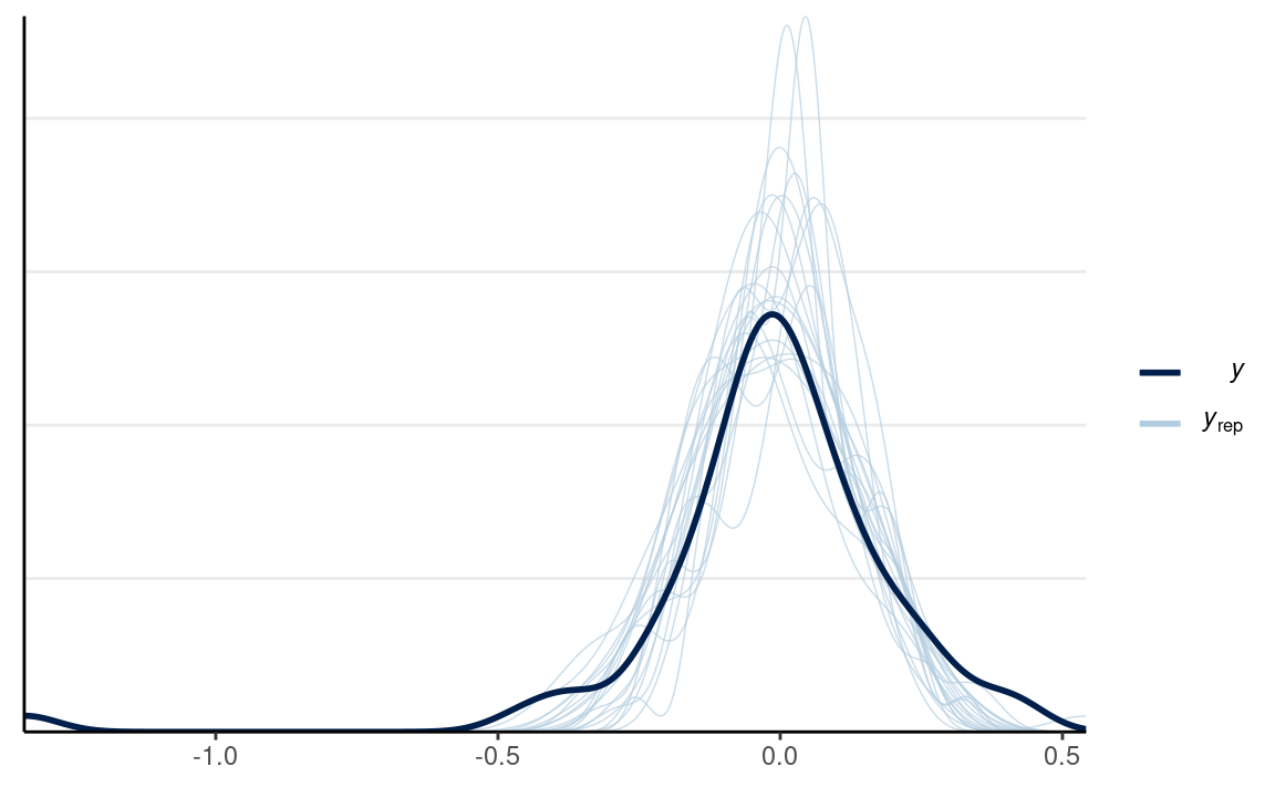
We can look at the posterior predictive distributions of the individual differences in response time across conditions
y1_tilde <- rstan::extract(m3, pars = "y1_rep")$y1_rep
y2_tilde <- rstan::extract(m3, pars = "y2_rep")$y2_rep
# Randomly sample 20 data sets (for faster plotting)
selected_rows <- sample.int(nrow(y1_tilde), size = 20)
ppc_dens_overlay(m3_dat$y2 - m3_dat$y1,
                 yrep = y2_tilde[selected_rows, ] - y1_tilde[selected_rows, ],
                 bw = "SJ")
Effect Size
An effect size measures the magnitude of a difference. When the unit of the outcome is meaningful, an unstandardized effect size should be used. In this case, the response is in seconds, but the parameter \(\delta\) is in the log unit. To convert things back to the original unit, we need to use the property that the expected value of a lognormal distribution is \(\exp(\mu + \sigma^2 / 2)\). Therefore, to obtain the mean difference between the two conditions in seconds, we have \[\exp(\mu_2 + \sigma^2 / 2) - \exp(\mu_1 + \sigma^2 / 2)\]
m3_draws <- as.array(m3, pars = c("mu1", "dmu", "sigma")) %>%
    as_draws_array() %>%
    mutate_variables(es = exp(mu1 + dmu + sigma^2 / 2) -
        exp(mu1 + sigma^2 / 2))
m3_summary <- summarise_draws(m3_draws)
So the mean difference estimate in seconds between the two conditions was -0.01 seconds, 90% CI [-0.05, 0.03].
Region of Practical Equivalence
One thing that is often of interest in research is establishing equivalence between two values. We may wonder, for example,
- whether an experimental manipulation has an effect size of zero (\(d\) = 0),
- whether two variables are truly uncorrelated (\(r\) = 0),
- whether the blood type distribution is the same across countries,
- whether two parallel forms of a test have the same difficulty level
Here in our example, we can investigate
Whether lying in native and second languages requires the same response time.
In all these above scenarios, we are interested in “confirming” whether a quantity is equal to another quantity. The traditional null hypothesis significance testing (NHST), however, won’t allow us to do that. That’s because NHST is set up to reject the null hypothesis, but failure to reject \(d\) = 0 does not confirm that \(d\) = 0; it just means that we don’t have enough evidence for that. In addition, we know in advance, with a high degree of certainty, that \(d\) \(\neq\) 0. Do we truly believe that the treatment group and the control group will perform exactly the same on an IQ test? Even when one group got 100 and the other 100.0000001, the null hypothesis is false.
Therefore, what we really meant when saying whether two things are equal is not whether two quantities are exactly the same, which is basically impossible, but whether two quantities are close enough, or practically equivalent. In the IQ test example, most of us would agree that the two groups are practically equivalent.
So what we actually want to test, in mathematical notation, is \[|\mu_2 - \mu_1| < \epsilon,\] where \(\epsilon\) is some small value of a difference by which \(\beta\) and \(\beta_0\) are deemed practically equivalent. For example, in our analysis, we may think that if the difference is less than .05 seconds (or 50ms), we may say that there is no difference in RT. In other words, if there is a high probability (in a Bayesian sense) that \[-\epsilon < \beta < \epsilon\] than we considered there is sufficient evident that \(\beta\) = \(\beta_0\) in a practical sense. The interval (\(-\epsilon\), \(\epsilon\)) is what your textbook author referred to as the region of practical equivalence, or ROPE.
Using ROPE, we accept the difference in two parameters is practically zero if there is a high probability that delta is within a region indistinguishable from zero.
Let’s compute the probability of the effect size being within [-50ms, 50ms]:
es_draws <- extract_variable(m3_draws, variable = "es")
mean(es_draws >= -.05 & es_draws <= .05)
#> [1] 0.964So there is a high probability that the mean difference is null.
Last updated
#> [1] "March 24, 2022"