Hamiltonian Monte Carlo
A more recent development in MCMC is the development of algorithms under the umbrella of Hamiltonian Monte Carlo or hybrid Monte Carlo (HMC). The algorithm is a bit complex, and my goal is to help you develop some intuition of the algorithm, hopefully, enough to help you diagnose the Markov chains.
- It produces simulation samples that are much less correlated, meaning that if you get 10,000 samples from Metropolis and 10,000 samples from HMC, HMC generally provides a much higher effective sample size (ESS).
- It does not require conjugate priors
- When there is a problem in convergence, HMC tends to raise a clear red flag, meaning it goes really, really wrong.
So now, how does HMC work? First, consider a two-dimensional posterior below, which is the posterior of \((\mu, \tau)\) from a normal model.
The HMC algorithm improves from the Metropolis algorithm by simulating smart proposal values. It does so by using the gradient of the logarithm of the posterior density. Let’s first take the log of the joint density:
Now, flip it up-side-down
Imagine placing a marble on the above surface. With gravity, it is natural that the marble will have a tendency to move to the bottom of the surface. If you place the marble in a higher location, it will have a higher potential energy and tends to move faster towards the bottom, because that energy converts to a larger kinetic energy. If you place it close to the bottom, it will tend to move slower.
For simplicity, let’s consider just one dimension with the following picture:
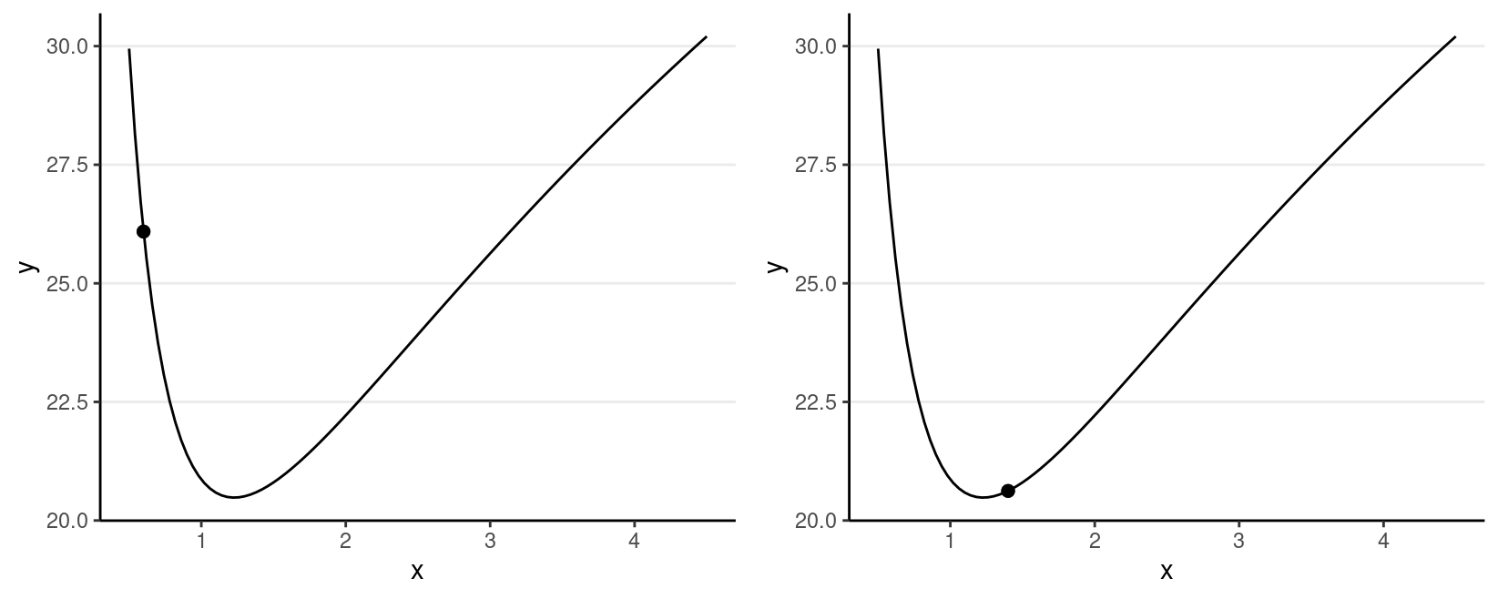
For the graph on the left, the marble (represented as a dot) has high potential energy and should quickly go down to the bottom; on the right, the marble has low potential energy and should move less fast.
Therefore, if the sampler is near the bottom (i.e., the point with high posterior density), it tends to stay there.
But we don’t want the marble to stay at the bottom without moving; otherwise, all our posterior draws will be just the posterior mode. In HMC, it moves the marble with a push, called momentum. The direction and the magnitude of the momentum will be randomly simulated, usually from a normal distribution. If the momentum is large, it should travel farther away; however, it also depends on the gradient, which is the slope in a one-dimension case.
HMC generates a proposed value by simulating the motion of an object on a surface, based on an initial momentum with a random magnitude and direction, and locating the object after a fixed amount of time.
At the beginning of a trajectory, the marble has a certain amount of kinetic energy and potential energy, and the sum is the total amount of energy, called the Hamiltonian. Based on the conservation of energy, at any point in the motion, the Hamiltonian should remain constant.
The following shows the trajectory of a point starting at 2, with a random momentum of 0.5 in the positive direction.
This one has the same starting value, with a random momentum of 0.5 in the negative direction.

Leapfrog Integrator
To simulate the marble’s motion, one needs to solve a system of differential equations, which is not an easy task. A standard method is to use the so-called leapfrog integrator, which discretizes a unit of time into \(L\)*$ steps. The following shows how it approximates the motion using \(L\) = 3 and \(L\) = 10 steps. The red dot is the target. As can be seen, larger \(L\) simulates the motion more accurately.

If the simulated trajectory is different from the true trajectory by a certain threshold, like the one on the left, it is called a divergent transition, in which case the proposed value should not be trusted. In software like STAN, it will print out a warning about that. When the number of divergent transitions is large, one thing to do is increase \(L\). If that does not help, it may indicate some difficulty in a high-dimensional model, and reparameterization may be needed.
In this course, you will use STAN to draw posterior samples. For more information on HMC, go to https://mc-stan.org/docs/2_28/reference-manual/hamiltonian-monte-carlo.html. You can also find some sample R code at http://www.stat.columbia.edu/~gelman/book/software.pdf.
The No-U-Turn Sampler (NUTS)
Although HMC is more efficient by generating smarter proposal values, one performance bottleneck is that the motion sometimes takes a U-turn, like in some graphs above, in which the marble goes up (right) and then goes down (left), and eventually may stay in a similar location. The improvement of NUTS is that it uses a binary search tree that simulates both the forward and backward trajectory. The algorithm is complex, but to my understanding, it achieves two purposes: (a) finding the path that avoids a U-turn and (b) selecting an appropriate number of leapfrog steps, \(L\). When each leapfrog step moves slowly, the search process may take a long time. With NUTS, one can control the maximum depth of the search tree.
See https://mc-stan.org/docs/2_28/reference-manual/hmc-algorithm-parameters.html for more information on NUTS
Introduction to STAN
The engine used for running the Bayesian analyses covered in this
course is STAN, as well as the rstan package
that allows it to interface with R. STAN requires some
programming from the users, but the benefit is that it allows users to
fit a lot of different kinds of models. The goal of this lecture is not
to make you an expert on STAN; instead, the goal is to give
you a brief introduction with some sample codes so that you can study
further by yourself, and know where to find the resources to write your
own models when you need to.
STAN (http://mc-stan.org/) is itself a programming language,
just like R. Strictly speaking, it is not only for Bayesian methods, as
you can actually do penalized maximum likelihood and automatic
differentiation, but it is most commonly used as an MCMC sampler for
Bayesian analyses. It is written in C++, which makes it much faster than
R (R is actually quite slow as a computational language). You can write
a STAN program without calling R or other software,
although eventually, you likely will need to use statistical software to
post-process the posterior samples after running MCMC. There are
interfaces of STAN for different programs, including R,
Python, MATLAB, Julia, Stata, and Mathematica, and for us, we will be
using the RStan interface.
STAN code
In STAN, you need to define a model using the
STAN language. Below is an example for a normal model,
which is saved with the file name "normal_model.stan".
data {
  int<lower=0> N;  // number of observations
  vector[N] y;  // data vector y
}
parameters {
  real mu;  // mean parameter
  real<lower=0> sigma;  // non-negative SD parameter
}
model {
  // model
  y ~ normal(mu, sigma);  // use vectorization
  // prior
  mu ~ normal(5, 10);
  sigma ~ student_t(4, 0, 3);
}
generated quantities {
  vector[N] y_rep;  // place holder
  for (n in 1:N)
    y_rep[n] = normal_rng(mu, sigma);
}
In STAN, anything after // denotes comments
and will be ignored by the program. In each block (e.g.,
data {}), a statement should end with a semicolon
(;). There are several blocks in the above
STAN code:
data: The data input forSTANis usually not only an R data frame, but a list that includes other information, such as sample size, number of predictors, and prior scales. Each type of data has an input type, such asint= integer,real= numbers with decimal places,matrix= 2-dimensional data of real numbers,vector= 1-dimensional data of real numbers, andarray= 1- to many-dimensional data. For exampley[N]is a one-dimensional array of integers.
you can set the lower and upper bounds so that
STANcan check the input dataparameters: The parameters to be estimatedtransformed parameters: optional variables that are transformations of the model parameters. It is usually used for more advanced models to allow more efficient MCMC sampling.model: It includes expressions of prior distributions for each parameter and the likelihood for the data. There are many possible distributions that can be used inSTAN.generated quantities: Any quantities that are not part of the model but can be computed from the parameters for every iteration. Examples include posterior generated samples, effect sizes, and log-likelihood (for fit computation).
RStan
STAN is written in C++, which is a compiled language.
This is different from programs like R, in which you can input command
and get results right away. In contrast, a STAN program
needs to be converted to something that can be executed on your
computer. The benefit, however, is that the programs can be run much
faster after the compilation process.
To feed data from R to STAN, and import output from
STAN to R, you will follow the steps to install the
rstan package (https://github.com/stan-dev/rstan/wiki/RStan-Getting-Started).
Revisiting the Note-Taking Example
We will revisit the note-taking example:
# Use haven::read_sav() to import SPSS data
nt_dat <- read_sav("https://osf.io/qrs5y/download")
(wc_laptop <- nt_dat$wordcount[nt_dat$condition == 0] / 100)
#>  [1] 4.20 4.61 5.72 4.47 3.34 1.27 2.65 3.40 2.43 2.55 2.73 2.26 3.16
#> [14] 2.47 3.25 1.67 4.49 4.77 1.67 5.19 3.00 2.98 1.59 2.23 4.39 2.29
#> [27] 1.52 2.13 3.11 3.82 2.62
Assemble data list in R
First, you need to assemble a list of data for STAN
input, which should match the specific STAN program. In the
STAN program we define two components (N and
`y’) for data, so we need these two elements in an R list:
Load rstan
library(rstan)
rstan_options(auto_write = TRUE)  # save compiled STAN object
Sampling the Prior
The priors used in the STAN code is \(\mu \sim N(0, 10)\) and \(\sigma \sim t^+_4(0, 3)\). To perform a prior predictive check, we can sample the prior. In STAN there’s no direct option to do it, but we can modify the STAN code to comment out the model part:
data {
  int<lower=0> N;  // number of observations
  vector[N] y;  // data vector y
}
parameters {
  real mu;  // mean parameter
  real<lower=0> sigma;  // non-negative SD parameter
}
model {
  // model
  // y ~ normal(mu, sigma);  // use vectorization
  // prior
  mu ~ normal(5, 10);
  sigma ~ student_t(4, 0, 3);
}
generated quantities {
  vector[N] y_rep;  // place holder
  for (n in 1:N)
    y_rep[n] = normal_rng(mu, sigma);
}
Then call stan()
We can extract the prior predictive draws, and plot the data:
set.seed(6)
y_tilde <- as.matrix(norm_prior, pars = "y_rep")
# Randomly sample 100 data sets (to make plotting faster)
selected_rows <- sample.int(nrow(y_tilde), size = 100)
ppc_dens_overlay(wc_laptop, yrep = y_tilde[selected_rows, ], bw = "SJ")

Sampling the Posterior
Summarize the results
After you call the stan function in R, it will compile
the STAN program, which usually takes a minute (but more
for more complex models). Then it starts sampling. You can now see a
summary of the results by printing the results:
#> Inference for Stan model: normal_model.
#> 4 chains, each with iter=2000; warmup=1000; thin=1;
#> post-warmup draws per chain=1000, total post-warmup draws=4000.
#>
#>       mean se_mean   sd 2.5%  25% 50%  75% 97.5% n_eff Rhat
#> mu    3.10       0 0.22 2.66 2.96 3.1 3.24  3.53  3161    1
#> sigma 1.21       0 0.16 0.95 1.10 1.2 1.31  1.59  3320    1
#>
#> Samples were drawn using NUTS(diag_e) at Thu Apr 28 11:40:22 2022.
#> For each parameter, n_eff is a crude measure of effective sample size,
#> and Rhat is the potential scale reduction factor on split chains (at
#> convergence, Rhat=1).
Table
You can use the posterior::summarize_draws() function to
get a table:
norm_fit %>%
    # Convert to `draws` object to work with the `posterior` package
    as_draws() %>%
    # Extract only mu and sigma
    subset_draws(variable = c("mu", "sigma")) %>%
    # Get summary
    summarize_draws() %>%
    # Use `knitr::kable()` for tabulation
    knitr::kable()
| variable | mean | median | sd | mad | q5 | q95 | rhat | ess_bulk | ess_tail |
|---|---|---|---|---|---|---|---|---|---|
| mu | 3.098351 | 3.103943 | 0.2219817 | 0.2134166 | 2.7369916 | 3.454369 | 1.001118 | 3206.011 | 2614.294 |
| sigma | 1.214441 | 1.196367 | 0.1622298 | 0.1549344 | 0.9846263 | 1.511318 | 1.000792 | 3406.807 | 2515.845 |
Plots
# Scatter plot matrix
mcmc_pairs(norm_fit, pars = c("mu", "sigma"))

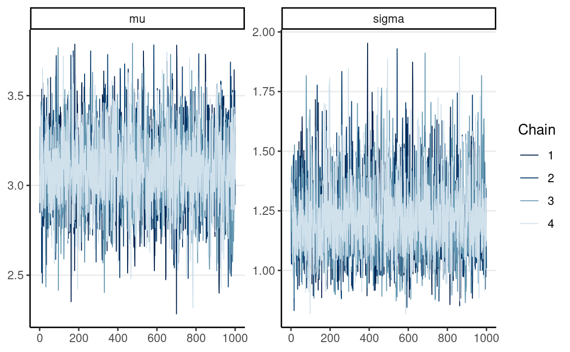
# Trace plots
mcmc_trace(norm_fit, pars = c("mu", "sigma"))
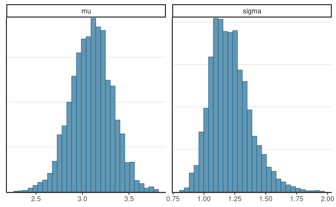
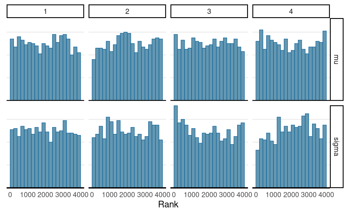
# Rank plots
mcmc_rank_hist(norm_fit, pars = c("mu", "sigma"))
And you can also use the shinystan package to visualize
the results:
shinystan::launch_shinystan(norm_fit)
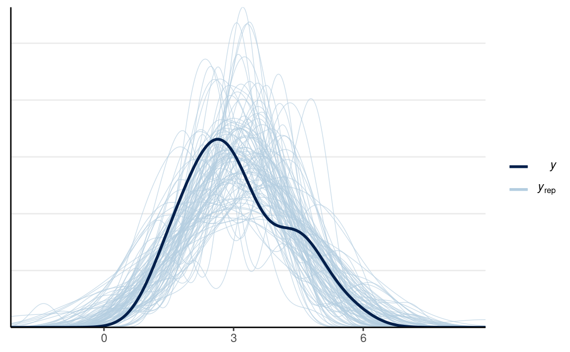
Posterior Predictive
We can extract the posterior predictive draws, and plot the data:
# Same code as prior predictive check
y_tilde <- as.matrix(norm_fit, pars = "y_rep")
# Randomly sample 100 data sets (to make plotting faster)
selected_rows <- sample.int(nrow(y_tilde), size = 100)
ppc_dens_overlay(wc_laptop, yrep = y_tilde[selected_rows, ], bw = "SJ")
Resources
STAN is extremely powerful and can fit almost any
statistical model, but the price is that it takes more effort to code
the model. To learn more about STAN, please check out https://mc-stan.org/users/documentation/ for the manual,
examples of some standard models, and case studies (including more
complex models like item response theory). Here are some case studies
that may be of interest to you:
- Regression (linear, logistic, ordered logistic): https://mc-stan.org/docs/2_29/stan-users-guide/linear-regression.html
- Item response theory: https://mc-stan.org/docs/2_29/stan-users-guide/item-response-models.html
- Time series: https://mc-stan.org/docs/2_29/stan-users-guide/time-series.html
- Meta-analysis: https://mc-stan.org/docs/2_29/stan-users-guide/meta-analysis.html
- Clustering models: https://mc-stan.org/docs/2_29/stan-users-guide/clustering.html
- Latent class model: https://mc-stan.org/users/documentation/case-studies/Latent_class_case_study.html
See https://cran.r-project.org/web/packages/rstan/vignettes/rstan.html
for a vignette for working with the rstan package.
Though fitting simple models in STAN may sometimes be
more work, for complex models, STAN could be a lifesaver as
it would be tough to fit some of those models with other approaches.
Things to pay attention for STAN:
- Define the type
- Define the bound
- End with a “;”
- Different format for a for loop
Last updated
#> [1] "March 10, 2022"