library(tidyverse)
library(here)  # for easier management of file paths
library(rstan)
rstan_options(auto_write = TRUE)  # save compiled Stan object
library(brms)  # simplify fitting Stan GLM models
library(posterior)  # for summarizing draws
library(bayesplot)  # for plotting
library(modelsummary)  # table for brms
theme_set(theme_classic() +
    theme(panel.grid.major.y = element_line(color = "grey92")))
Binary Logistic Regression
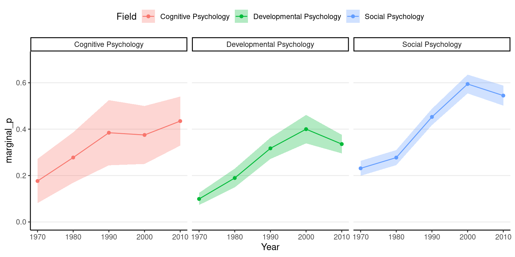
We will use an example from this paper (https://journals.sagepub.com/doi/abs/10.1177/0956797616645672), which examines how common it was for researchers to report marginal \(p\) values (i.e., .05 < \(p\) \(\leq\) .10). The outcome is whether a study reported one or more marginal \(p\) values (1 = Yes, 0 = No). The researchers also categorized the studies into three subfields (Cognitive Psychology, Developmental Psychology, Social Psychology), and there were a total of 1,535 studies examined from 1970 to 2010.
# readxl package can be used to import excel files
datfile <- here("data_files", "marginalp.xlsx")
if (!file.exists(datfile)) {
    dir.create(here("data_files"))
    download.file("https://osf.io/r4njf/download",
        destfile = datfile
    )
}
marginalp <- readxl::read_excel(datfile)
# Recode `Field` into a factor
marginalp <- marginalp %>%
    # Filter out studies without any experiments
    filter(`Number of Experiments` >= 1) %>%
    mutate(Field = factor(Field,
        labels = c(
            "Cognitive Psychology",
            "Developmental Psychology",
            "Social Psychology"
        )
    )) %>%
    # Rename the outcome
    rename(marginal_p = `Marginals Yes/No`)
# Proportion of marginal p in each subfield across Years
marginalp %>%
    ggplot(aes(x = Year, y = marginal_p)) +
    stat_summary(aes(fill = Field), geom = "ribbon", alpha = 0.3) +
    stat_summary(aes(col = Field), geom = "line") +
    stat_summary(aes(col = Field), geom = "point") +
    coord_cartesian(ylim = c(0, 0.7)) +
    facet_wrap(~ Field) +
    theme(legend.position = "top")
Centering
The issue of centering applies for most regression models, including
GLMs. Because the predictor Year has values 1970, 1980,
etc, if we use this variable as a predictor, the intercept \(\beta_0\) will be the predicted value of
\(\eta\) when Year = 0,
which is like 2,000 years before the data were collected. So instead, we
usually want the value 0 to be something meaningful and/or a possible
value in the data. So we will center the variable year by making 0 the
year 1970. In addition, we will divide the values by 10 so that one unit
in the new predictor means 10 years.
In other words, we will use a transformed predictor,
Year10 = (Year - 1970) / 10. So when
Year = 1970, Year10 = 10; when
Year = 1990, Year10 = 2.
marginalp <- marginalp %>%
  mutate(Year10 = (Year - 1970) / 10)
# Check the recode
distinct(marginalp, Year, Year10)
#> # A tibble: 5 × 2
#>    Year Year10
#>   <dbl>  <dbl>
#> 1  1980      1
#> 2  1970      0
#> 3  2000      3
#> 4  1990      2
#> 5  2010      4
For this example, I’ll look at the subset for developmental psychology. You may want to try with the other subsets of the data for practice.
#> # A tibble: 6 × 9
#>   Field        `Paper Title` Authors  Year `Number of Exp…` marginal_p
#>   <fct>        <chr>         <chr>   <dbl>            <dbl>      <dbl>
#> 1 Development… A New Look a… Christ…  2010                1          1
#> 2 Development… A Tale to Tw… daniel…  2010                1          1
#> 3 Development… Associations… Rachel…  2010                1          1
#> 4 Development… Attachment-b… kathyr…  2000                1          1
#> 5 Development… Effects of A… Timoth…  1990                1          1
#> 6 Development… Effortful co… grazyn…  2000                1          1
#> # … with 3 more variables: `First or Only Marginal` <dbl>,
#> #   `Conventional Threshold` <dbl>, Year10 <dbl>
Model and Priors
As the name “logistic regression” suggested, the logistic function is used somewhere in the model. The logistic function, or the inverse logit function, is \[\mu = g^{-1}(\eta) = \frac{\exp(\eta)}{1 + \exp(\eta)},\] which is a transformation from \(\eta\) to \(\mu\). The link function, which is a transformation from \(\mu\) to \(\eta\), is the logit function, \[\eta = g(\mu) = \log\frac{\mu}{1 - \mu},\] which converts \(\mu\), which is in probability metric, to \(\eta\), which is in log odds metric (odds = probability / [1 - probability]).
Model:
\[\begin{align} \text{marginal_p}_i & \sim \mathrm{Bern}(\mu_i) \\ \log(\mu_i) & = \eta_i \\ \eta_i & = \beta_0 + \beta_1 \text{Year10}_{i} \end{align}\]
Priors:
\[\begin{align} \beta_0 & \sim t_4(0, 2.5) \\ \beta_1 & \sim t_4(0, 1) \end{align}\]
There has been previous literature on what choices of prior on the \(\beta\) coefficients for logistic regressions would be appropriate (see this paper). \(\beta\) coefficients in logistic regression can be relatively large, unlike in normal regression. Therefore, it’s pointed out that a heavy tail distribution, like Cauchy and \(t\), would be more appropriate. Recent discussions have settled on priors such as \(t\) distributions with a small degrees of freedom as a good balance between heavy tails and efficiency for MCMC sampling. I use \(t_4(4, 0, 2.5)\) for \(\beta_0\), which puts more density to be in [-2.5, 2.5] on the log odds unit. This means, in the year 1970, our belief is that the probability of marginally significant results would be somewhere between 0.0758582 to 0.9241418, which seems to cover a reasonable range. For \(\beta_1\), I use \(t_4(4, 0, 1)\), which suggests that a 10 year difference like corresponds to a difference in log odds between -1 and 1. While it’s hard to interpret difference in log odds, a quick rule of thumb is to divide \(\beta_1\) by 4, which roughly corresponds to the maximum difference in probability for unit difference in the predictor. So if \(\beta_1\) = 1, the maximum difference in probability will be no more than 25 percentage points. So my prior says that it’s unlikely that the probability of reporting marginal \(p\) values would increase or decrease by 25 percentage points every 10 years, which again is a weak prior. If you’re uncertain, you can consider something weaker.
The priors are chosen to be weakly informative.
Note that in brms we used
family = bernoulli(). In other R functions, such as
glm, they do not distinguish between bernoulli and Binomial
and only recognize family = binomial(), as a Bernoulli
variable is a binomial variable with \(n =
1\).
Interpreting the results
Any non-linear relationships will involve more work in interpretations, and the coefficients in logistic regressions are no exceptions.
Posterior predictions
A good way to start is to plot the model-implied association on the
original unit of the data. The conditional_effects()
function in brms comes in very handy, and I recommend you
always start with that:
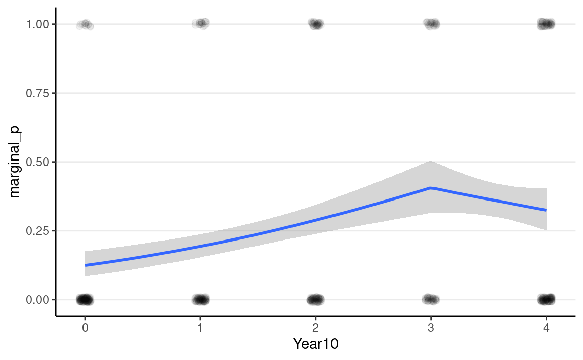
plot(
    conditional_effects(m4, prob = .90),
    points = TRUE,
    point_args = list(height = 0.01, width = 0.05, alpha = 0.05)
)
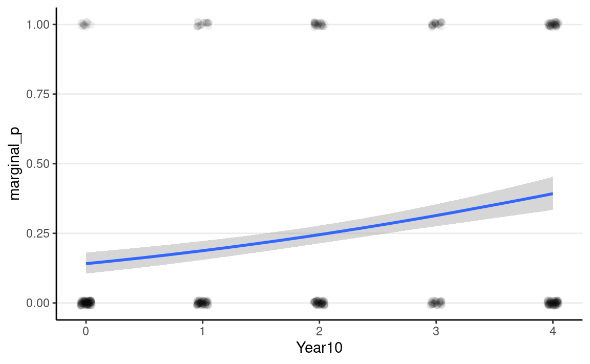
As you can see, the logistic model implies a somewhat non-linear
association between Year10 and the outcome. From the graph,
when Year10 = 2, which is the Year 1990, the predicted
probability of marginal significant results is about 25%, with a 90%
credible interval of about 21 to 28%. We can get that using
posterior_epred(m4, newdata = list(Year10 = 2)) %>%
    summarise_draws()
#> # A tibble: 1 × 10
#>   variable  mean median     sd    mad    q5   q95  rhat ess_bulk
#>   <chr>    <dbl>  <dbl>  <dbl>  <dbl> <dbl> <dbl> <dbl>    <dbl>
#> 1 ...1     0.246  0.245 0.0193 0.0190 0.214 0.278  1.00    5651.
#> # … with 1 more variable: ess_tail <dbl>
Intercept
From the equation, when all predictors are zero, we have \[\mathrm{logit}(\mu_i) = \beta_0.\]
Therefore, the intercept is the log odds that a study reported a
marginally significant \(p\) value when
Year10 = 0 (i.e, in 1970), which was estimated to be -1.81,
90% CI [-2.14, -1.51]. As log odds are not as intuitive as probability,
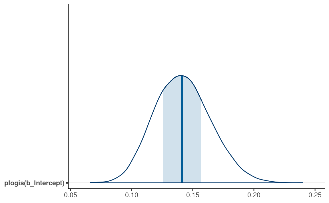
it is common to instead interpret \(\hat{\mu}
= \mathrm{logistic}(\beta_0)\), which is the conditional
probability of being marginal_p = 1 in 1970. For Bayesian,
that means obtaining the posterior distribution of \(\mathrm{logistic}(\beta_0)\), which can be
done by
m4_draws <- as_draws_array(m4)
m4_draws <- m4_draws %>%
    mutate_variables(logistic_beta0 = plogis(b_Intercept))
summarize_draws(m4_draws)
#> # A tibble: 5 × 10
#>   variable         mean   median     sd    mad       q5      q95  rhat
#>   <chr>           <dbl>    <dbl>  <dbl>  <dbl>    <dbl>    <dbl> <dbl>
#> 1 b_Intercept    -1.81    -1.81  0.191  0.194    -2.14    -1.51   1.00
#> 2 b_Year10        0.344    0.343 0.0687 0.0689    0.231    0.458  1.00
#> 3 lprior         -3.08    -3.08  0.0410 0.0406   -3.15    -3.02   1.00
#> 4 lp__         -295.    -295.    1.01   0.726  -297.    -294.     1.00
#> 5 logistic_be…    0.142    0.141 0.0229 0.0234    0.106    0.181  1.00
#> # … with 2 more variables: ess_bulk <dbl>, ess_tail <dbl>
The bayesplot package allow you to plot transformed
parameters quickly:
mcmc_areas(m4, pars = "b_Intercept",
           transformations = list("b_Intercept" = "plogis"),
           bw = "SJ")
Interpreting \(\exp(\beta_1)\) as odds ratio
The slope, \(\beta_1\), represents
the difference in the predicted log odds between two observations with 1
unit difference in the predictor. For example, for two individuals with
1 unit difference in Year10 (i.e., 10 years), we have \[\mathrm{logit}(\mu_{\text{marginal_p} = 1}) -
\mathrm{logit}(\mu_{\text{marginal_p} = 0}) = \beta_1.\]
Again, difference in log odds are hard to interpret, and so we will exponentiate to get \[\frac{\mathrm{odds}_{\text{marginal_p} = 1}} {\mathrm{odds}_{\text{marginal_p} = 0}} = \exp(\beta_1).\]
The fraction on the left hand side is the odds ratio of
reporting a marginal \(p\) value
associated with a one unit difference in Year10 (i.e., 10
years). An odds of 1.0 means that the probability of success and failure
is equal; an odds > 1 means success is more likely than failures; and
an odds < 1 means success is less likely than failures. Again, for
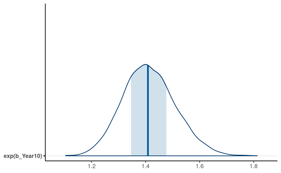
Bayesian, we can obtain the posterior distribution of \(\exp(\beta_1)\) by
m4_draws <- m4_draws %>%
    mutate_variables(exp_beta1 = exp(b_Year10))
summarize_draws(m4_draws)
#> # A tibble: 6 × 10
#>   variable         mean   median     sd    mad       q5      q95  rhat
#>   <chr>           <dbl>    <dbl>  <dbl>  <dbl>    <dbl>    <dbl> <dbl>
#> 1 b_Intercept    -1.81    -1.81  0.191  0.194    -2.14    -1.51   1.00
#> 2 b_Year10        0.344    0.343 0.0687 0.0689    0.231    0.458  1.00
#> 3 lprior         -3.08    -3.08  0.0410 0.0406   -3.15    -3.02   1.00
#> 4 lp__         -295.    -295.    1.01   0.726  -297.    -294.     1.00
#> 5 logistic_be…    0.142    0.141 0.0229 0.0234    0.106    0.181  1.00
#> 6 exp_beta1       1.41     1.41  0.0974 0.0970    1.26     1.58   1.00
#> # … with 2 more variables: ess_bulk <dbl>, ess_tail <dbl>
Using the posterior mean, we predict that the odds of reporting a marginal \(p\) value for a study that is 10 years later is multiplied by 0.14 times, 90% CI [0.11, 0.18]; in other words, every 10 years, the odds increased by -85.8139207%. Here’s the posterior density plot for the odds ratio:
mcmc_areas(m4, pars = "b_Year10",
           transformations = list("b_Year10" = "exp"),
           bw = "SJ")
Odds ratio (OR) is popular as the multiplicative effect is constant, thus making interpretations easier. Also, in medical research and some other research areas, OR can be an excellent approximation of the relative risk, which is the probability ratio of two groups, of some rare disease or events. However, odds and odds ratio are never intuitive metrics for people, and in many situations a large odds ratio may be misleading as it corresponds to a very small effect. Therefore, in general I would recommend you to interpret coefficients in probability unit, even though that means more work.
Interpreting Coefficients in Probability Units
Another way to interpret the results of logistic regression
coefficient is to examine the change in probability. Because the
predicted probability is a non-linear function of the predictors, a one
unit difference in the predictor has different meanings depending on the
values on \(X\) you chose for
interpretations. You can see that in the
conditional_effects() plot earlier.
Consider the change in the predicted probability of reporting a
marginal \(p\) value with
Year10 = 0 (1970), Year10 = 1 (1980), to
Year10 = 4, respectively:
m4_pred <- posterior_epred(m4, list(Year10 = 0:4))
colnames(m4_pred) <- paste0("Year10=", 0:4)
summarise_draws(m4_pred)
#> # A tibble: 5 × 10
#>   variable  mean median     sd    mad    q5   q95  rhat ess_bulk
#>   <chr>    <dbl>  <dbl>  <dbl>  <dbl> <dbl> <dbl> <dbl>    <dbl>
#> 1 Year10=0 0.142  0.141 0.0229 0.0234 0.106 0.181  1.00    4503.
#> 2 Year10=1 0.188  0.188 0.0208 0.0209 0.155 0.223  1.00    4674.
#> 3 Year10=2 0.246  0.245 0.0193 0.0190 0.214 0.278  1.00    5651.
#> 4 Year10=3 0.314  0.314 0.0240 0.0236 0.276 0.354  1.00    7305.
#> 5 Year10=4 0.393  0.393 0.0363 0.0363 0.334 0.453  1.00    6868.
#> # … with 1 more variable: ess_tail <dbl>
As you can see, the predicted difference in probability is smaller
when comparing Year10 = 0 and 1, but is larger when
comparing Year10 = 3 and 4.
The “divide by 4 rule”
A quick approximation is to divide the coefficient by 4 to get an
upper bound on the change in probability associated with a one unit
change in the predictor. In our example, this corresponds to 0.3437533 /
4 = 0.0859383, which is very close to the predicted difference in
probability from Year10 = 3 to Year10 = 4.
Posterior Predictive Check
pp_check(
    m4,
    type = "error_binned"
)
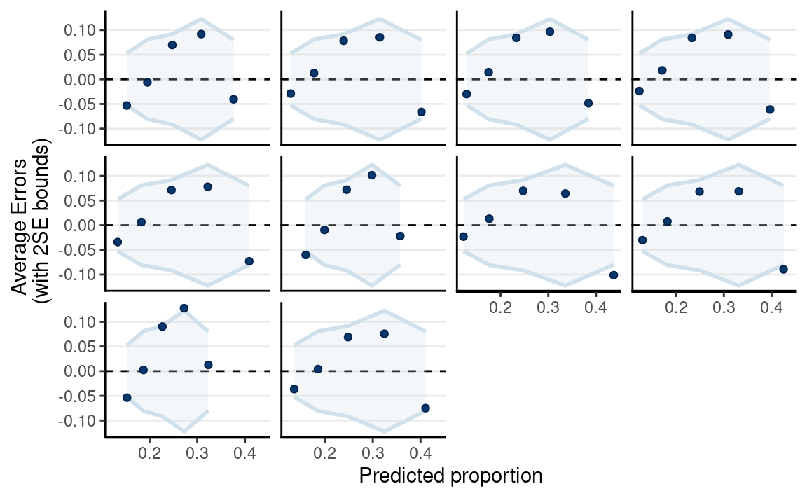
The linear model is not the best fit.
Linear Spline
Use bs() to specify a linear spline (degree = 1) with
one turning point (knots = 3).
Posterior Prediction
plot(
    conditional_effects(m5),
    points = TRUE,
    point_args = list(height = 0.01, width = 0.05, alpha = 0.05)
)
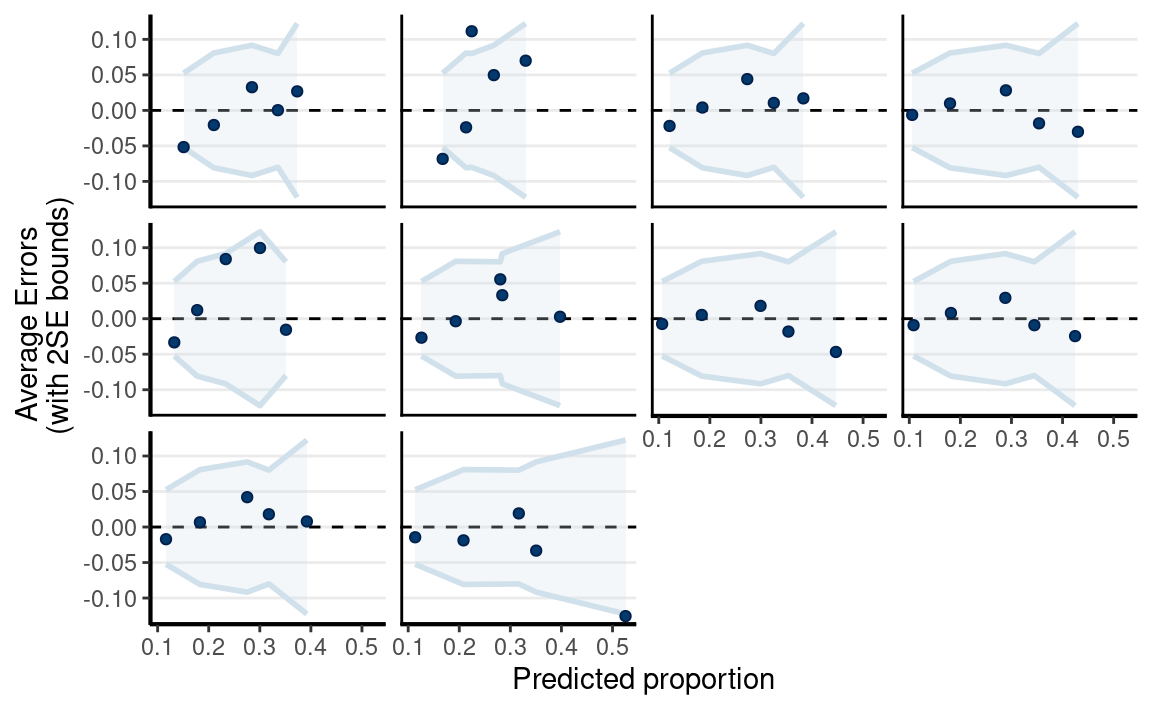
pp_check(
    m5,
    type = "error_binned",
    x = "Year10"
)
Model Comparison
msummary(list(linear = m4, `linear spline` = m5),
         estimate = "{estimate} [{conf.low}, {conf.high}]",
         statistic = NULL, fmt = 2)
| linear | linear spline | |
|---|---|---|
| b_Intercept | −1.81 [−2.19, −1.45] | −1.95 [−2.36, −1.52] |
| b_Year10 | 0.34 [0.21, 0.48] | |
| b_bsYear10degreeEQ1knotsEQ31 | 1.57 [0.95, 2.27] | |
| b_bsYear10degreeEQ1knotsEQ32 | 1.22 [0.69, 1.79] | |
| Num.Obs. | 535 | 535 |
| ELPD | −292.9 | −290.1 |
| ELPD s.e. | 11.2 | 11.1 |
| LOOIC | 585.9 | 580.3 |
| LOOIC s.e. | 22.4 | 22.2 |
| WAIC | 585.9 | 580.3 |
| RMSE | 0.43 | 0.42 |
The linear spline is better according to information criteria.
Binomial Logistic Regression
- Individual data: Bernoulli
- Grouped data: Binomial
The two above are equivalent
Model
\[\begin{align} \text{marginal_p}_j & \sim \mathrm{Bin}(N_j, \mu_j) \\ \log(\mu_j) & = \eta_j \\ \eta_j & = \beta_0 + \beta_1 \text{Year10}_{j} \end{align}\]
Priors:
\[\begin{align} \beta_0 & \sim t_3(0, 2.5) \\ \beta_1 & \sim t_4(0, 1) \end{align}\]
pp_check(m5_bin, type = "intervals", x = "Year10")
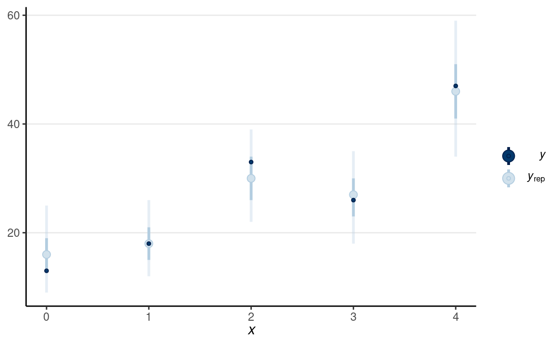
(#fig:ppc-m5_bin)Posterior predictive check using the predicted and observed counts.
Ordinal Regression
Check out this paper: https://journals.sagepub.com/doi/full/10.1177/2515245918823199
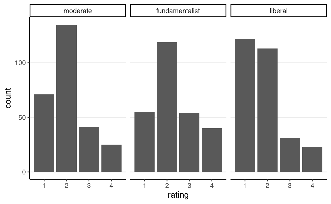
stemcell %>%
    ggplot(aes(x = rating)) +
    geom_bar() +
    facet_wrap(~ belief)
https://www.thearda.com/archive/files/Codebooks/GSS2006_CB.asp
The outcome is attitude towards stem cells research, and the predictor is religious belief.
Recently, there has been controversy over whether the government should provide any funds at all for scientific research that uses stem cells taken from human embryos. Would you say the government . . .
- 1 = Definitely, should fund such research
- 2 = Probably should fund such research
- 3 = Probably should not fund such research
- 4 = Definitely should not fund such research
Model
\[\begin{align} \text{rating}_i & \sim \mathrm{Categorical}(\pi^1_i, \pi^2_i, \pi^3_i, \pi^4_i) \\ \pi^1_{i} & = \mathrm{logit}^{-1}(\tau^1 - \eta_i) \\ \pi^2_{i} & = \mathrm{logit}^{-1}(\tau^2 - \eta_i) - \mathrm{logit}^{-1}(\tau^1 - \eta_i) \\ \pi^3_{i} & = \mathrm{logit}^{-1}(\tau^3 - \eta_i) - \mathrm{logit}^{-1}(\tau^2 - \eta_i) \\ \pi^4_{i} & = 1 - \mathrm{logit}^{-1}(\tau^3 - \eta_i) \\ \eta_i & = \beta_1 \text{fundamentalist}_{i} + \beta_2 \text{liberal}_{i} \end{align}\]
Priors:
\[\begin{align} \tau^1, \tau^2, \tau^3 & \sim t_3(0, 2.5) \\ \beta_1 & \sim N(0, 1) \end{align}\]
m6 <- brm(
    rating ~ belief,
    data = stemcell,
    family = cumulative(link = "logit"),
    prior = prior(std_normal(), class = "b")
)
Posterior Predictive Check
pp_check(m6, type = "bars_grouped", group = "belief",
         ndraws = 100)
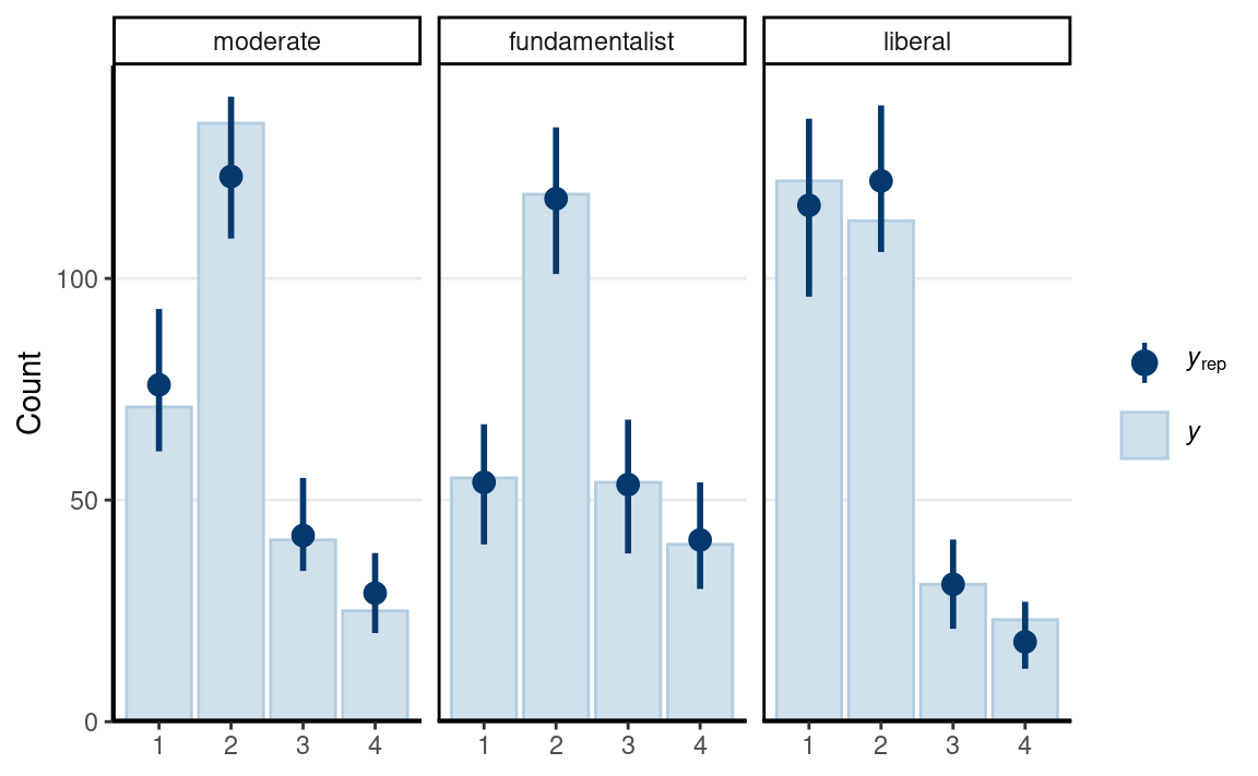
The fit was reasonable.
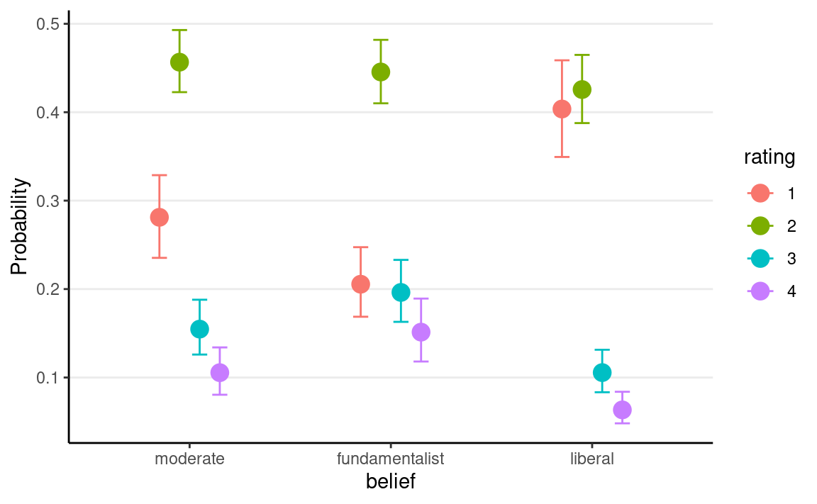
Plot
conditional_effects(m6, categorical = TRUE)
Nominal Logistic Regression
Ordinal regression is a special case of nominal regression with the proportional odds assumption.
Model
\[\begin{align} \text{rating}_i & \sim \mathrm{Categorical}(\pi^1_{i}, \pi^2_{i}, \pi^3_{i}, \pi^4_{i}) \\ \pi^1_{i} & = \frac{1}{\exp(\eta^2_{i}) + \exp(\eta^3_{i}) + \exp(\eta^4_{i}) + 1} \\ \pi^2_{i} & = \frac{\exp(\eta^2_{i})}{\exp(\eta^2_{i}) + \exp(\eta^3_{i}) + \exp(\eta^4_{i}) + 1} \\ \pi^3_{i} & = \frac{\exp(\eta^3_{i})}{\exp(\eta^2_{i}) + \exp(\eta^3_{i}) + \exp(\eta^4_{i}) + 1} \\ \pi^4_{i} & = \frac{\exp(\eta^4_{i})}{\exp(\eta^2_{i}) + \exp(\eta^3_{i}) + \exp(\eta^4_{i}) + 1} \\ \eta^2_{i} & = \beta^2_{0} + \beta^2_{1} \text{fundamentalist}_{i} + \beta^2_{2} \text{liberal}_{i} \\ \eta^3_{i} & = \beta^3_{0} + \beta^3_{1} \text{belief}_{i} + \beta^3_{2} \text{liberal}_{i} \\ \eta^4_{i} & = \beta^4_{0} + \beta^4_{1} \text{belief}_{i} + \beta^4_{2} \text{liberal}_{i} \\ \end{align}\]
As you can see, it has two additional parameters for each predictor column.
m7 <- brm(
    rating ~ belief,
    data = stemcell,
    family = categorical(link = "logit"),
    prior = prior(std_normal(), class = "b", dpar = "mu2") +
        prior(std_normal(), class = "b", dpar = "mu3") +
        prior(std_normal(), class = "b", dpar = "mu4")
)
Model Comparison
msummary(list(`ordinal (proportional odds)` = m6, norminal = m7),
         estimate = "{estimate} [{conf.low}, {conf.high}]",
         statistic = NULL, fmt = 2)
| ordinal (proportional odds) | norminal | |
|---|---|---|
| b_Intercept[1] | −0.94 [−1.17, −0.71] | |
| b_Intercept[2] | 1.04 [0.80, 1.27] | |
| b_Intercept[3] | 2.14 [1.86, 2.43] | |
| b_belieffundamentalist | 0.41 [0.08, 0.70] | |
| b_beliefliberal | −0.55 [−0.85, −0.24] | |
| b_mu2_Intercept | 0.63 [0.35, 0.90] | |
| b_mu3_Intercept | −0.57 [−0.94, −0.22] | |
| b_mu4_Intercept | −1.06 [−1.47, −0.61] | |
| b_mu2_belieffundamentalist | 0.12 [−0.30, 0.53] | |
| b_mu2_beliefliberal | −0.69 [−1.07, −0.33] | |
| b_mu3_belieffundamentalist | 0.52 [0.00, 1.01] | |
| b_mu3_beliefliberal | −0.76 [−1.31, −0.22] | |
| b_mu4_belieffundamentalist | 0.70 [0.16, 1.29] | |
| b_mu4_beliefliberal | −0.58 [−1.15, 0.00] | |
| Num.Obs. | 829 | 829 |
| ELPD | −1019.3 | −1020.9 |
| ELPD s.e. | 15.5 | 15.6 |
| LOOIC | 2038.6 | 2041.9 |
| LOOIC s.e. | 31.0 | 31.2 |
| WAIC | 2038.6 | 2041.8 |
Last updated
#> [1] "April 16, 2022"