One Parameter ModelsPSYC 573University of Southern CaliforniaFebruary 01, 20221 / 30

2 / 30

An Example of Bernoulli Data3 / 30

Data (Subsample)Patients diagnosed with AIDS in Australia before 1 July 1991


state
sex
diag
death
status
T.categ
age


VIC
M
1991-03-05
1991-07-01
A
hs
36

NSW
M
1987-08-30
1988-03-11
D
hs
25

QLD
M
1989-10-09
1990-08-22
D
hs
36

NSW
M
1991-03-17
1991-07-01
A
hs
42

NSW
M
1986-04-12
1989-01-31
D
hs
40

NSW
M
1986-09-29
1987-03-25
D
hs
69

NSW
M
1989-08-24
1991-07-01
A
hs
37

Other
F
1988-10-19
1991-07-01
A
id
30

NSW
M
1990-04-07
1991-01-21
D
hs
30

NSW
M
1988-04-28
1990-04-07
D
hs
41


4 / 30

state	sex	diag	death	status	T.categ	age
VIC	M	1991-03-05	1991-07-01	A	hs	36
NSW	M	1987-08-30	1988-03-11	D	hs	25
QLD	M	1989-10-09	1990-08-22	D	hs	36
NSW	M	1991-03-17	1991-07-01	A	hs	42
NSW	M	1986-04-12	1989-01-31	D	hs	40
NSW	M	1986-09-29	1987-03-25	D	hs	69
NSW	M	1989-08-24	1991-07-01	A	hs	37
Other	F	1988-10-19	1991-07-01	A	id	30
NSW	M	1990-04-07	1991-01-21	D	hs	30
NSW	M	1988-04-28	1990-04-07	D	hs	41

5 / 30

Image credit: Wikimedia Commons

5 / 30

Image credit: Wikimedia Commons

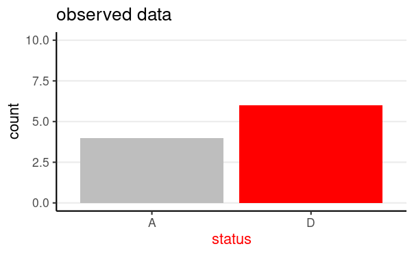
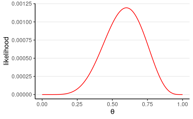
Let's go through the Bayesian crank

5 / 30

Image credit: Wikimedia Commons

Choose a Model: Bernoulli

Data: $y$ = survival status (0 = "A", 1 = "D")

Parameter: $θ$ = probability of "D"

Model equation: $y_{i} \sim Bern (θ)$ for $i = 1, 2, \dots, N$

The model states:

the sample data $y$ follows a Bernoulli distribution with the common parameter $θ$

6 / 30

Bernoulli Likelihood

Notice that there is no subscript for $θ$ :

The model assumes each observation has the same $θ$
I.e., the observations are exchangeable

$P (y_{1}, y_{2}, \dots, y_{N}) = θ^{z} (1 - θ)^{N - z}$

$z$ = number of "successes" ("D")

$z$ = 6 in this illustrative sample

7 / 30

theta	likelihood
0.0	0.00000
0.1	0.00000
0.2	0.00003
0.3	0.00018
0.4	0.00053
0.5	0.00098
0.6	0.00119
0.7	0.00095
0.8	0.00042
0.9	0.00005
1.0	0.00000

8 / 30

Choosing Priors9 / 30

Specify a Prior

When choosing priors, start with the support of the parameter(s)

Values that are possible

Support for $θ$ : [0, 1]

10 / 30

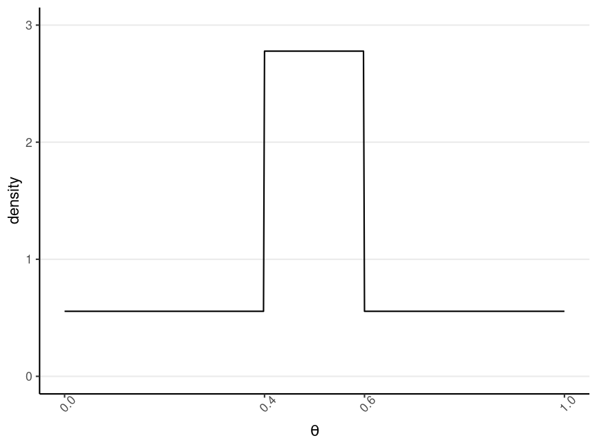
One Possible Option

Prior belief: $θ$ is most likely to be in the range $[.40, .60)$ , and is 5 times more likely than any values outside of that range"

11 / 30

Conjugate Prior: Beta Distribution

$P (θ ∣ a, b) \propto θ^{a - 1} (1 - θ)^{b - 1} I_{[0, 1]}$

a <- 1
b <- 1
dbeta(theta1, shape1 = a, shape2 = b)

Conjugate Prior: yield posterior in the same distribution family as the prior

Some other conjugate distributions: https://en.wikipedia.org/wiki/Conjugate_prior#Table_of_conjugate_distributions

12 / 30

Two hyperparameters, $a$ and $b$ :

$a - 1$ = number of prior 'successes' (e.g., "D")
$b - 1$ = number of prior 'failures'

13 / 30

When $a > b$ , more density to the right (i.e., larger $θ$ ), and vice versa

Mean = $a / (a + b)$

Concentration = $κ = a + b$ ; $↑ κ$ , $↓$ variance, $↑$ strength of prior

E.g., A Beta(1, 1) prior means 0 prior success and 0 failure

i.e., no prior information (i.e., noninformative)

14 / 30

Notes on Choosing Priors

Give $>$ 0 probability/density for all possible values of a parameter
When the prior contains relatively little information
- different choices usually make little difference
Do a prior predictive check
Sensitivity analyses to see how sensitive results are to different reasonable prior choices.

15 / 30

Getting the Posterior16 / 30

Obtaining the Posterior Analytically

$P (θ ∣ y) = \frac{P (y ∣ θ) P (θ)}{\int_{0}^{1} P (y ∣ θ^{*}) P (θ^{*}) d θ^{*}}$

The denominator is usually intractable

17 / 30

Obtaining the Posterior Analytically

$P (θ ∣ y) = \frac{P (y ∣ θ) P (θ)}{\int_{0}^{1} P (y ∣ θ^{*}) P (θ^{*}) d θ^{*}}$

The denominator is usually intractable

Conjugate prior: Posterior is from a known distribution family

$N$ trials and $z$ successes
$B e t a (a, b)$ prior
$\Rightarrow$ $B e t a (a + z, b + N - z)$ posterior
- $a + z - 1$ successes
- $b + N - z - 1$ failures

17 / 30

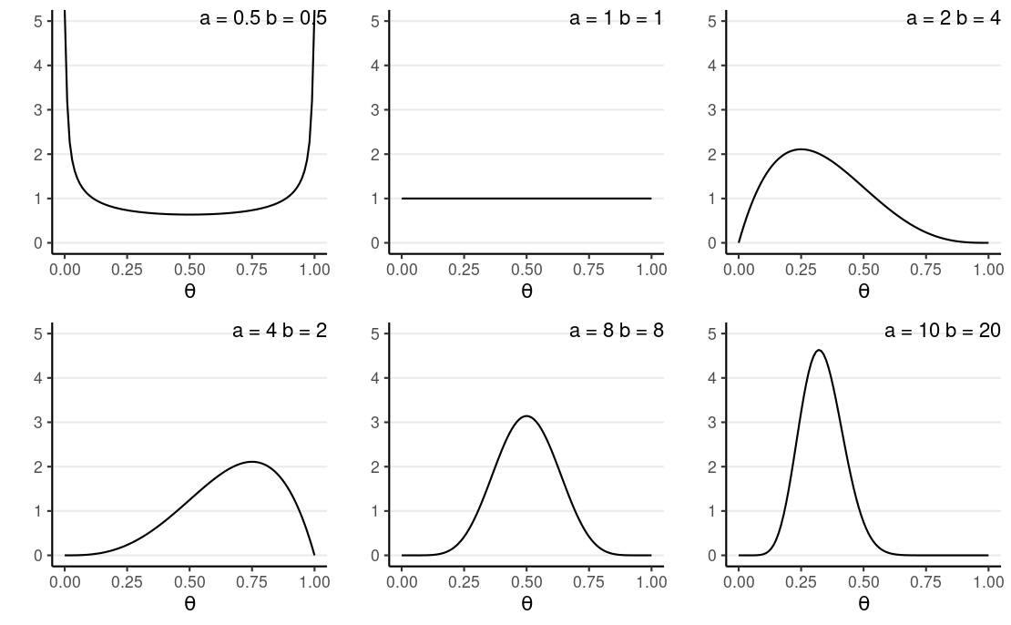
Back to the Example

$N$ = 10, $z$ = 6

Prior: Do you believe that the fatality rate of AIDS is 100%? or 0%?

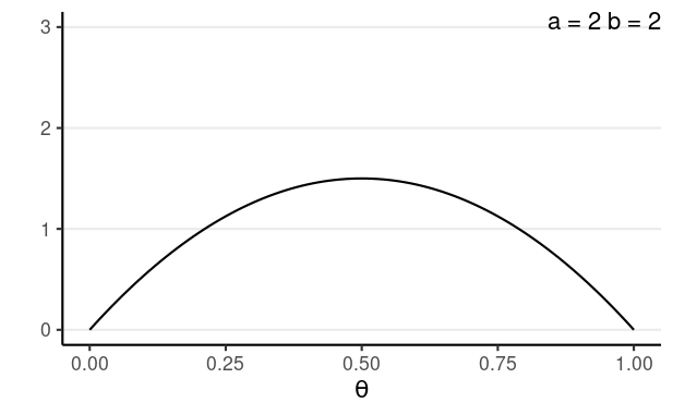
Let's use $κ = 4$ , prior mean = 0.5, so $a$ = 2 and $b$ = 2

18 / 30

Posterior Beta

$θ ∣ y \sim B e t a (2 + 6, 2 + 4)$

ggplot(tibble(x = c(0, 1)), aes(x = x)) +
    stat_function(fun = dbeta,
                  args = list(shape1 = 8, shape2 = 6)) +
    labs(title = "Beta(a = 8, b = 6)",
         x = expression(theta), y = "Density")

19 / 30

Summarizing the Posterior

If the posterior is from a known family, one can evalue summary statistics analytically

E.g., $E (θ ∣ y) = \int_{0}^{1} θ P (θ ∣ y) d θ$

However, more often, a simulation-based approach is used to draw samples from the posterior

num_draws <- 1000
sim_theta <- rbeta(1000, shape1 = 8, shape2 = 6)

20 / 30

Statistic
Common name
Value


mean
Bayes estimate/Expected a posteriori (EAP)
0.563

median
Posterior median
0.567

mode
Maximum a posteriori (MAP)
0.577

SD
Posterior SD
0.126

MAD
MAD
0.13

80% CI
(Equal-tailed) Credible interval
[0.398, 0.727]

80% HDI
HDI/Highest Posterior Density Interval (HPDI)
[0.404, 0.733]

21 / 30

Statistic	Common name	Value
mean	Bayes estimate/Expected a posteriori (EAP)	0.563
median	Posterior median	0.567
mode	Maximum a posteriori (MAP)	0.577
SD	Posterior SD	0.126
MAD	MAD	0.13
80% CI	(Equal-tailed) Credible interval	[0.398, 0.727]
80% HDI	HDI/Highest Posterior Density Interval (HPDI)	[0.404, 0.733]

Use the Full Data

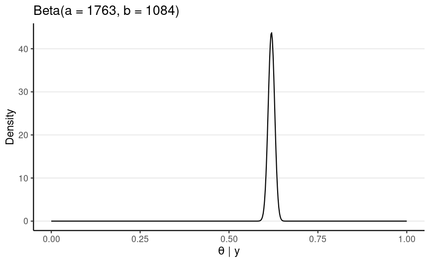
1082 A, 1761 D $\to$ $N$ = 2843, $z$ = 1761

Posterior: Beta(1763, 1084)

22 / 30

Posterior Predictive Check23 / 30

Posterior Predictive Check

$\tilde{y}$ = new/future data

Posterior predictive: $P (\tilde{y} ∣ y) = \int P (\tilde{y} ∣ θ, y) P (θ ∣ y) d θ$

24 / 30

Posterior Predictive Check

$\tilde{y}$ = new/future data

Posterior predictive: $P (\tilde{y} ∣ y) = \int P (\tilde{y} ∣ θ, y) P (θ ∣ y) d θ$

Simulate $θ^{*}$ from posterior --> for each $θ^{*}$ , simulate a new data set

24 / 30

Posterior Predictive Check

$\tilde{y}$ = new/future data

Posterior predictive: $P (\tilde{y} ∣ y) = \int P (\tilde{y} ∣ θ, y) P (θ ∣ y) d θ$

Simulate $θ^{*}$ from posterior --> for each $θ^{*}$ , simulate a new data set

If the model does not fit the data, any results are basically meaningless at best, and can be very misleading

Requires substantive knowledge and some creativity

E.g., are the case fatality rates equal across the 4 state categories?

24 / 30

25 / 30

Posterior Predictive Check

Some common checks:

Does the model simulate data with similar distributions as the observed data?
- e.g., skewness, range
Subsets of observed data that are of more interest?
- e.g., old age group
- If not fit, age should be incorporated in the model

See an example in Gabry et al. (2019)

26 / 30

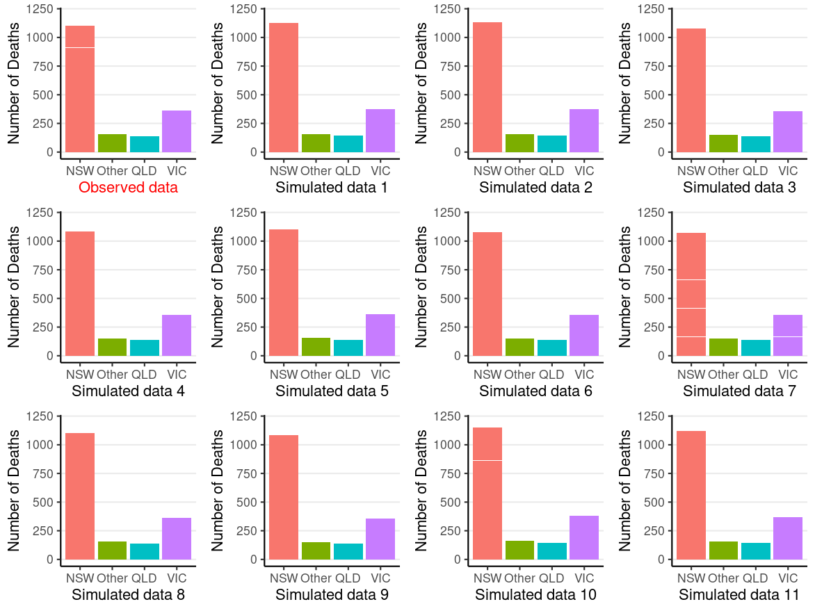
Using `bayesplot`

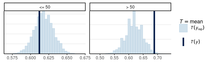
Darker line = observed proportion of "D"; histogram = simulated plausible statistics based on the model and the posterior

The model with one-parameter, which assumes exchangeability, does not fit those age 50+

May need more than one $θ$

# Create an age group indicator
age50 <- factor(Aids2$age > 50, labels = c("<= 50", "> 50"))
# Draw posterior samples of theta
post_sample <- rbeta(1e4, 1807, 1116)
# Initialize an S by N matrix to store the simulated data
y_tilde <- matrix(NA,
                  nrow = length(post_sample),
                  ncol = length(Aids2$status))
for (s in seq_along(post_sample)) {
    theta_s <- post_sample[s]
    status_new <- sample(c("D", "A"), nrow(Aids2),
        replace = TRUE,
        prob = c(theta_s, 1 - theta_s)
    )
    y_tilde[s,] <- as.numeric(status_new == "D")
}
bayesplot::ppc_stat_grouped(
    as.numeric(Aids2$status == "D"),
    yrep = y_tilde,
    group = age50
)

27 / 30

Other One-Parameter Models28 / 30

Binomial ModelFor count outcome: yi∼Bin(Ni,θ)yi∼Bin(Ni,θ)θθ: rate of occurrence (per trial)

Conjugate prior: Beta
E.g.,yy minority candidates in NN new hires
yy out of NN symptoms checked
A word appears yy times in a tweet of NN number of words

29 / 30

Poisson ModelFor count outcome: yi∼Pois(θ)yi∼Pois(θ)θθ: rate of occurrence

Conjugate prior: Gamma
E.g., Drinking yy times in a week
yy hate crimes in a year for a county
yy people visiting a store in an hour

30 / 30

↑, ←, Pg Up, k	Go to previous slide
↓, →, Pg Dn, Space, j	Go to next slide
Home	Go to first slide
End	Go to last slide
Number + Return	Go to specific slide
b / m / f	Toggle blackout / mirrored / fullscreen mode
c	Clone slideshow
p	Toggle presenter mode
t	Restart the presentation timer
?, h	Toggle this help

One Parameter Models

PSYC 573

University of Southern California

February 01, 2022

An Example of Bernoulli Data

Data (Subsample)

Choose a Model: Bernoulli

Bernoulli Likelihood

Choosing Priors

Specify a Prior

One Possible Option

Conjugate Prior: Beta Distribution

Notes on Choosing Priors

Getting the Posterior

Obtaining the Posterior Analytically

Obtaining the Posterior Analytically

Back to the Example

Posterior Beta

Summarizing the Posterior

Use the Full Data

Posterior Predictive Check

Posterior Predictive Check

Posterior Predictive Check

Posterior Predictive Check

Posterior Predictive Check

Using bayesplot

Other One-Parameter Models

Binomial Model

Poisson Model

Help

Using `bayesplot`