Markov Chain Monte Carlo III
PSYC 573
University of Southern California
February 24, 2022
Hamiltonian Monte Carlo (HMC)
From Hamiltonian mechanics
- Use gradients to generate better proposal values
Results:
- Higher acceptance rate
- Less autocorrelation/higher ESS
- Better suited for high dimensional problems
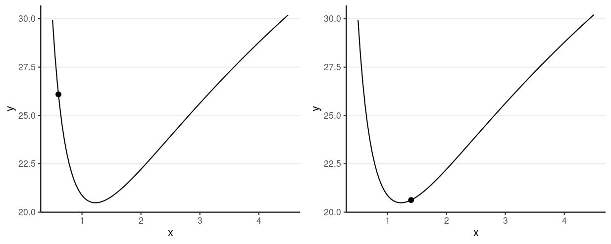
Gradients of Log Density
Consider just σ2
Potential energy = −logP(θ)
Which one has a higher potential energy?
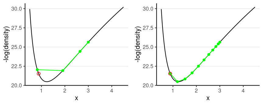
HMC Algorithm
Imagine a marble on a surface like the log posterior
- Simulate a random momentum (usually from a normal distribution)
- Apply the momentum to the marble to roll on the surface
- Treat the position of the marble after some time as the proposed value
- Accept the new position based on the Metropolis step
- i.e., probabilistically using the posterior density ratio
Leapfrog Integrator
Location and velocity constantly change
Leapfrog integrator
- Solve for the new location using L leapfrog steps
- Larger L, more accurate location
- Higher curvature requires larger L and smaller step size
Divergent transition: When the leapfrog approximation deviates substantially from where it should be
No-U-Turn Sampler (NUTS)
Algorithm used in STAN
Two problems of HMC
- Need fine-tuning L and step size
- Wasted steps when the marble makes a U-turn
No-U-Turn Sampler (NUTS)
Algorithm used in STAN
Two problems of HMC
- Need fine-tuning L and step size
- Wasted steps when the marble makes a U-turn
NUTS uses a binary search tree to determine L and the step size
- The maximum treedepth determines how far it searches
See a demo here: https://chi-feng.github.io/mcmc-demo/app.html
Stan
Stan
A language for doing MCMC sampling (and other related methods, such as maximum likelihood estimation)
Current version (2.29): mainly uses NUTS
Stan
A language for doing MCMC sampling (and other related methods, such as maximum likelihood estimation)
Current version (2.29): mainly uses NUTS
It supports a wide range of distributions and prior distributions
Written in C++ (faster than R)
Consider the example
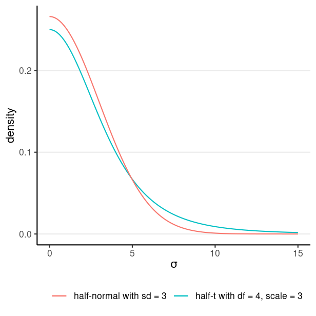
Model: wc_laptopi∼N(μ,σ) Prior: μ∼N(5,10)σ∼t+4(0,3)
t+4(0,3) is a half-t distribution with df = 4 and scale = 3
An example STAN model
data { int<lower=0> N; // number of observations vector[N] y; // data vector y}parameters { real mu; // mean parameter real<lower=0> sigma; // non-negative SD parameter}model { // model y ~ normal(mu, sigma); // use vectorization // prior mu ~ normal(5, 10); sigma ~ student_t(4, 0, 3);}generated quantities { vector[N] y_rep; // place holder for (n in 1:N) y_rep[n] = normal_rng(mu, sigma);}Components of a STAN Model
data: Usually a list of different typesint,real,matrix,vector,array
can set lower/upper bounds
parameterstransformed parameters: optional variables that are transformation of the model parametersmodel: definition of priors and the likelihoodgenerated quantities: new quantities from the model (e.g., simulated data)
RStan
https://mc-stan.org/users/interfaces/rstan
An interface to call Stan from R, and import results from STAN to R
Call rstan
library(rstan)rstan_options(auto_write = TRUE) # save compiled STAN objectnt_dat <- haven::read_sav("https://osf.io/qrs5y/download")wc_laptop <- nt_dat$wordcount[nt_dat$condition == 0] / 100# Data: a list with names matching the Stan programnt_list <- list( N = length(wc_laptop), # number of observations y = wc_laptop # outcome variable (yellow card))# Call Stannorm_prior <- stan( file = here("stan", "normal_model.stan"), data = nt_list, seed = 1234 # for reproducibility)># ># SAMPLING FOR MODEL 'normal_model' NOW (CHAIN 1).># Chain 1: ># Chain 1: Gradient evaluation took 7e-06 seconds># Chain 1: 1000 transitions using 10 leapfrog steps per transition would take 0.07 seconds.># Chain 1: Adjust your expectations accordingly!># Chain 1: ># Chain 1: ># Chain 1: Iteration: 1 / 2000 [ 0%] (Warmup)># Chain 1: Iteration: 200 / 2000 [ 10%] (Warmup)># Chain 1: Iteration: 400 / 2000 [ 20%] (Warmup)># Chain 1: Iteration: 600 / 2000 [ 30%] (Warmup)># Chain 1: Iteration: 800 / 2000 [ 40%] (Warmup)># Chain 1: Iteration: 1000 / 2000 [ 50%] (Warmup)># Chain 1: Iteration: 1001 / 2000 [ 50%] (Sampling)># Chain 1: Iteration: 1200 / 2000 [ 60%] (Sampling)># Chain 1: Iteration: 1400 / 2000 [ 70%] (Sampling)># Chain 1: Iteration: 1600 / 2000 [ 80%] (Sampling)># Chain 1: Iteration: 1800 / 2000 [ 90%] (Sampling)># Chain 1: Iteration: 2000 / 2000 [100%] (Sampling)># Chain 1: ># Chain 1: Elapsed Time: 0.018408 seconds (Warm-up)># Chain 1: 0.016197 seconds (Sampling)># Chain 1: 0.034605 seconds (Total)># Chain 1: ># ># SAMPLING FOR MODEL 'normal_model' NOW (CHAIN 2).># Chain 2: ># Chain 2: Gradient evaluation took 5e-06 seconds># Chain 2: 1000 transitions using 10 leapfrog steps per transition would take 0.05 seconds.># Chain 2: Adjust your expectations accordingly!># Chain 2: ># Chain 2: ># Chain 2: Iteration: 1 / 2000 [ 0%] (Warmup)># Chain 2: Iteration: 200 / 2000 [ 10%] (Warmup)># Chain 2: Iteration: 400 / 2000 [ 20%] (Warmup)># Chain 2: Iteration: 600 / 2000 [ 30%] (Warmup)># Chain 2: Iteration: 800 / 2000 [ 40%] (Warmup)># Chain 2: Iteration: 1000 / 2000 [ 50%] (Warmup)># Chain 2: Iteration: 1001 / 2000 [ 50%] (Sampling)># Chain 2: Iteration: 1200 / 2000 [ 60%] (Sampling)># Chain 2: Iteration: 1400 / 2000 [ 70%] (Sampling)># Chain 2: Iteration: 1600 / 2000 [ 80%] (Sampling)># Chain 2: Iteration: 1800 / 2000 [ 90%] (Sampling)># Chain 2: Iteration: 2000 / 2000 [100%] (Sampling)># Chain 2: ># Chain 2: Elapsed Time: 0.020357 seconds (Warm-up)># Chain 2: 0.015692 seconds (Sampling)># Chain 2: 0.036049 seconds (Total)># Chain 2: ># ># SAMPLING FOR MODEL 'normal_model' NOW (CHAIN 3).># Chain 3: ># Chain 3: Gradient evaluation took 4e-06 seconds># Chain 3: 1000 transitions using 10 leapfrog steps per transition would take 0.04 seconds.># Chain 3: Adjust your expectations accordingly!># Chain 3: ># Chain 3: ># Chain 3: Iteration: 1 / 2000 [ 0%] (Warmup)># Chain 3: Iteration: 200 / 2000 [ 10%] (Warmup)># Chain 3: Iteration: 400 / 2000 [ 20%] (Warmup)># Chain 3: Iteration: 600 / 2000 [ 30%] (Warmup)># Chain 3: Iteration: 800 / 2000 [ 40%] (Warmup)># Chain 3: Iteration: 1000 / 2000 [ 50%] (Warmup)># Chain 3: Iteration: 1001 / 2000 [ 50%] (Sampling)># Chain 3: Iteration: 1200 / 2000 [ 60%] (Sampling)># Chain 3: Iteration: 1400 / 2000 [ 70%] (Sampling)># Chain 3: Iteration: 1600 / 2000 [ 80%] (Sampling)># Chain 3: Iteration: 1800 / 2000 [ 90%] (Sampling)># Chain 3: Iteration: 2000 / 2000 [100%] (Sampling)># Chain 3: ># Chain 3: Elapsed Time: 0.018081 seconds (Warm-up)># Chain 3: 0.017181 seconds (Sampling)># Chain 3: 0.035262 seconds (Total)># Chain 3: ># ># SAMPLING FOR MODEL 'normal_model' NOW (CHAIN 4).># Chain 4: ># Chain 4: Gradient evaluation took 4e-06 seconds># Chain 4: 1000 transitions using 10 leapfrog steps per transition would take 0.04 seconds.># Chain 4: Adjust your expectations accordingly!># Chain 4: ># Chain 4: ># Chain 4: Iteration: 1 / 2000 [ 0%] (Warmup)># Chain 4: Iteration: 200 / 2000 [ 10%] (Warmup)># Chain 4: Iteration: 400 / 2000 [ 20%] (Warmup)># Chain 4: Iteration: 600 / 2000 [ 30%] (Warmup)># Chain 4: Iteration: 800 / 2000 [ 40%] (Warmup)># Chain 4: Iteration: 1000 / 2000 [ 50%] (Warmup)># Chain 4: Iteration: 1001 / 2000 [ 50%] (Sampling)># Chain 4: Iteration: 1200 / 2000 [ 60%] (Sampling)># Chain 4: Iteration: 1400 / 2000 [ 70%] (Sampling)># Chain 4: Iteration: 1600 / 2000 [ 80%] (Sampling)># Chain 4: Iteration: 1800 / 2000 [ 90%] (Sampling)># Chain 4: Iteration: 2000 / 2000 [100%] (Sampling)># Chain 4: ># Chain 4: Elapsed Time: 0.018265 seconds (Warm-up)># Chain 4: 0.018438 seconds (Sampling)># Chain 4: 0.036703 seconds (Total)># Chain 4: