Hierarchical Models
PSYC 573
University of Southern California
March 3, 2022
Therapeutic Touch Example (N = 28)
Data Points From One Person
y: whether the guess of which hand was hovered over was correct
Person S01
| y | s |
|---|---|
| 1 | S01 |
| 0 | S01 |
| 0 | S01 |
| 0 | S01 |
| 0 | S01 |
| 0 | S01 |
| 0 | S01 |
| 0 | S01 |
| 0 | S01 |
| 0 | S01 |
Binomial Model
We can use a Bernoulli model: yi∼Bern(θ) for i=1,…,N
Binomial Model
We can use a Bernoulli model: yi∼Bern(θ) for i=1,…,N
Assuming exchangeability given θ, more succint to write z∼Bin(N,θ) for z=∑Ni=1yi
Binomial Model
We can use a Bernoulli model: yi∼Bern(θ) for i=1,…,N
Assuming exchangeability given θ, more succint to write z∼Bin(N,θ) for z=∑Ni=1yi
- Bernoulli: Individual trial
- Binomial: total count of "1"s
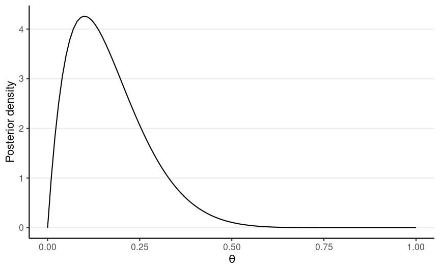
1 success, 9 failures
Posterior: Beta(2, 10)
Multiple People
We could repeat the binomial model for each of the 28 participants, to obtain posteriors for θ1, …, θ28
But . . .
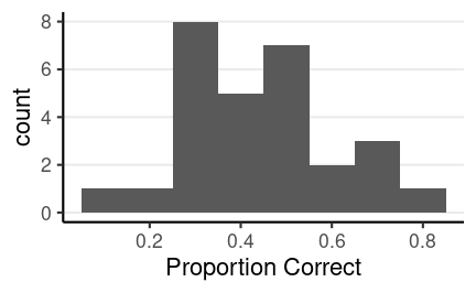
We'll continue the therapeutic touch example. To recap, we have 28 participants, each of them go through 10 trials to guess which of their hands was hovered above. The histogram shows the distribution of the proportion correct.
Multiple People
We could repeat the binomial model for each of the 28 participants, to obtain posteriors for θ1, …, θ28
But . . .
Do we think our belief about θ1 would inform our belief about θ2, etc?
After all, human beings share 99.9% of genetic makeup
We'll continue the therapeutic touch example. To recap, we have 28 participants, each of them go through 10 trials to guess which of their hands was hovered above. The histogram shows the distribution of the proportion correct.
Three Positions of Pooling
No pooling: each individual is completely different; inference of θ1 should be independent of θ2, etc
Complete pooling: each individual is exactly the same; just one θ instead of 28 θj's
Partial pooling: each individual has something in common but also is somewhat different
No Pooling
Complete Pooling
Partial Pooling
Partial Pooling in Hierarchical Models
Hierarchical Priors: θj∼Beta2(μ,κ)
Beta2: reparameterized Beta distribution
- mean μ=a/(a+b)
- concentration κ=a+b
Expresses the prior belief:
Individual θs follow a common Beta distribution with mean μ and concentration κ
How to Choose κ
If κ→∞: everyone is the same; no individual differences (i.e., complete pooling)
If κ=0: everybody is different; nothing is shared (i.e., no pooling)
How to Choose κ
If κ→∞: everyone is the same; no individual differences (i.e., complete pooling)
If κ=0: everybody is different; nothing is shared (i.e., no pooling)
We can fix a κ value based on our belief of how individuals are similar or different
How to Choose κ
If κ→∞: everyone is the same; no individual differences (i.e., complete pooling)
If κ=0: everybody is different; nothing is shared (i.e., no pooling)
We can fix a κ value based on our belief of how individuals are similar or different
A more Bayesian approach is to treat κ as an unknown, and use Bayesian inference to update our belief about κ
Generic prior by Kruschke (2015): κ ∼ Gamma(0.01, 0.01)
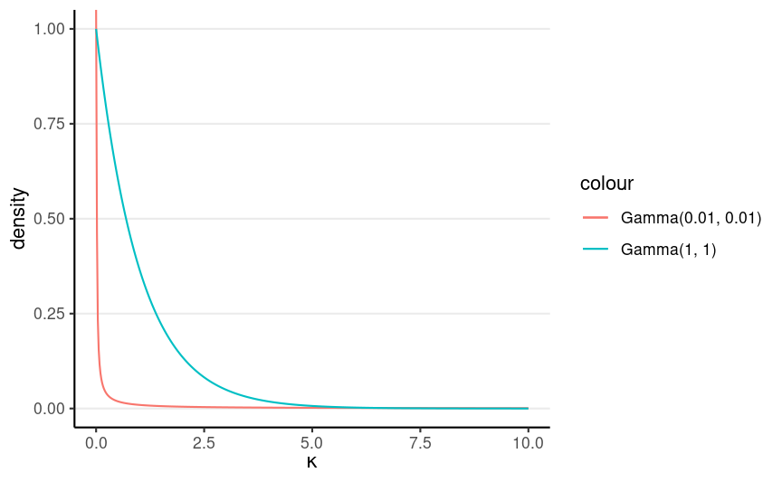
Sometimes you may want a stronger prior like Gamma(1, 1), if it is unrealistic to do no pooling
Full Model
Model: zj∼Bin(Nj,θj)θj∼Beta2(μ,κ) Prior: μ∼Beta(1.5,1.5)κ∼Gamma(0.01,0.01)
data { int<lower=0> J; // number of clusters (e.g., studies, persons) int y[J]; // number of "1"s in each cluster int N[J]; // sample size for each cluster}parameters { vector<lower=0, upper=1>[J] theta; // cluster-specific probabilities real<lower=0, upper=1> mu; // overall mean probability real<lower=0> kappa; // overall concentration}model { y ~ binomial(N, theta); // each observation is binomial theta ~ beta_proportion(mu, kappa); // prior; Beta2 dist mu ~ beta(1.5, 1.5); // weak prior kappa ~ gamma(.01, .01); // prior recommended by Kruschke}Here is the Stan code. The inputs are J, the number of people, y, which is actually z in our model for the individual counts, but I use y just because y is usually the outcome in Stan. N is the number of trials per person, and here N[J] means the number of trials can be different across individuals.
The parameters and the model block pretty much follow the mathematical model. The beta_proportion() function is what I said Beta2 as the beta distribution with the mean and the concentration as the parameters.
You may want to pause here to make sure you understand the Stan code.
Posterior of Hyperparameters
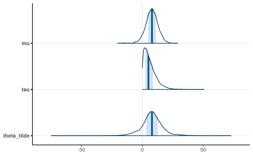
library(bayesplot)mcmc_dens(tt_fit, pars = c("mu", "kappa"))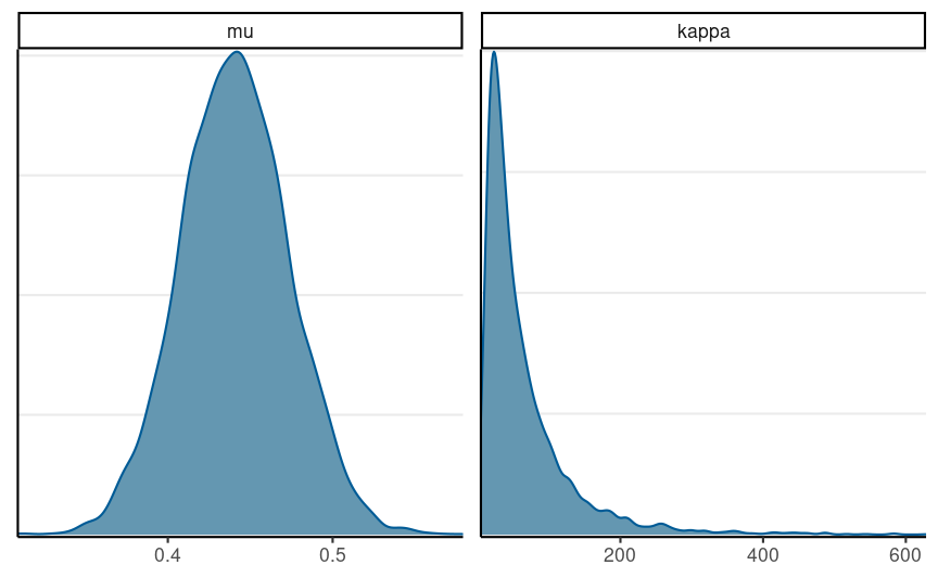
The graphs show the posterior for mu and kappa. As you can see, the average probability of guessing correctly has most density between .4 and .5.
For kappa, the posterior has a pretty long tail, and the value of kappa being very large, like 100 or 200, is pretty likely. So this suggests the individuals may be pretty similar to each other.
Shrinkage
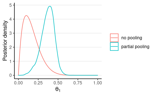
From the previous model, we get posterior distributions for all parameters, including mu, kappa, and 28 thetas. The first graph shows the posterior for theta for person 1. The red curve is the one without any pooling, so the distribution is purely based on the 10 trials for person 1. The blue curve, on the other hand, is much closer to .5 due to partial pooling. Because the posterior of kappa is pretty large, the posterior is pooled towards the grand mean, mu.
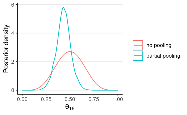
For the graph below, the posterior mean is close to .5 with or without partial pooling, but the distribution is narrower with partial pooling, which reflects a stronger belief. This is because, with partial pooling, the posterior distribution uses more information than just the 10 trials of person 15; it also borrows information from the other 27 individuals.
Multiple Comparisons?
Frequentist: family-wise error rate depends on the number of intended contrasts
One advantage of the hierarchical model is it is a solution to the multiple comparison problem. In frequentist analysis, if you have multiple groups, and you want to test each contrast, you will need to consider family-wise error rate, and do something like Bonferroni corrections.
Multiple Comparisons?
Frequentist: family-wise error rate depends on the number of intended contrasts
Bayesian: only one posterior; hierarchical priors already express the possibility that groups are the same
One advantage of the hierarchical model is it is a solution to the multiple comparison problem. In frequentist analysis, if you have multiple groups, and you want to test each contrast, you will need to consider family-wise error rate, and do something like Bonferroni corrections.
The Bayesian alternative is to do a hierarchial model with partial pooling. With Bayesian, you have one posterior distribution, which is the joint distribution of all parameters. And the use of a common distribution of the thetas already assigns some probability to the prior belief that the groups are the same.
Multiple Comparisons?
Frequentist: family-wise error rate depends on the number of intended contrasts
Bayesian: only one posterior; hierarchical priors already express the possibility that groups are the same
Thus, Bayesian hierarchical model "completely solves the multiple comparisons problem."1
[2]: See more in ch 11.4 of Kruschke (2015)
One advantage of the hierarchical model is it is a solution to the multiple comparison problem. In frequentist analysis, if you have multiple groups, and you want to test each contrast, you will need to consider family-wise error rate, and do something like Bonferroni corrections.
The Bayesian alternative is to do a hierarchial model with partial pooling. With Bayesian, you have one posterior distribution, which is the joint distribution of all parameters. And the use of a common distribution of the thetas already assigns some probability to the prior belief that the groups are the same.
Therefore, with a hierarchical model, you can obtain the posterior of the difference of any groups, without worrying about how many comparisons you have conducted. You can read more in the sources listed here.
Hierarchical Normal Model
In this video, we'll talk about another Bayesian hierarchical model, the hierarchical normal model.
Effect of coaching on SAT-V
| School | Treatment Effect Estimate | Standard Error |
|---|---|---|
| A | 28 | 15 |
| B | 8 | 10 |
| C | -3 | 16 |
| D | 7 | 11 |
| E | -1 | 9 |
| F | 1 | 11 |
| G | 18 | 10 |
| H | 12 | 18 |
The data come from the 1980s when scholars were debating the effect of coaching on standardized tests. The test of interest is the SAT verbal subtest. The note contains more description of it.
The analysis will be on the secondary data from eight schools, from school A to school H. Each schools conducts its own randomized trial. The middle column shows the treatment effect estimate for the effect of coaching. For example, for school A, we see that students with coaching outperformed students without coaching by 28 points. However, for schools C and E, the effects were smaller and negative.
Finally, in the last column, we have the standard error of the treatment effect for each school, based on a t-test. As you know, the smaller the standard error, the less uncertainty we have on the treatment effect.
Model: dj∼N(θj,sj)θj∼N(μ,τ) Prior: μ∼N(0,100)τ∼t+4(0,100)
data { int<lower=0> J; // number of schools real y[J]; // estimated treatment effects real<lower=0> sigma[J]; // s.e. of effect estimates }parameters { real mu; // overall mean real<lower=0> tau; // between-school SD vector[J] eta; // standardized deviation (z score)}transformed parameters { vector[J] theta; theta = mu + tau * eta; // non-centered parameterization}model { eta ~ std_normal(); // same as eta ~ normal(0, 1); y ~ normal(theta, sigma); // priors mu ~ normal(0, 100); tau ~ student_t(4, 0, 100);}Individual-School Treatment Effects
Prediction Interval
Posterior distribution of the true effect size of a new study, ~θ
See https://onlinelibrary.wiley.com/doi/abs/10.1002/jrsm.12 for an introductory paper on random-effect meta-analysis